Example: Lorenz system of differential equations

About the model

This tutorial shows how to perform uncertainty and sensitivity analysis of systems of differential equations with pygpc. In the following, we will analyse the Lorenz system. The governing equations are given by:

\[ \begin{align}\begin{aligned}\frac{\partial x}{\partial t} &= \sigma (y - x)\\\frac{\partial y}{\partial t} &= x (\rho - z) - y\\\frac{\partial z}{\partial t} &= xy - \beta z\end{aligned}\end{align} \]

The equations are implemented in the testfunction Lorenz system. The system is capable of showing chaotic behaviour and arises from simplified models for physical phenomena of lasers, electric circuits, thermodynamics and more. It returns time dependent x, y and z coordinates For each time point is treated as an independent quantity of interest and a separate gPC is performed to investigate the temporal evolutions of the uncertainties. The parameters \(\sigma\), \(\beta\) and \(\rho\) are usually assumed to be positive. Lorenz used the values \(\sigma=10\), \(\beta=8/3\), and \(\rho=28\). In the present example, they are assumed to be uncertain in defined ranges.

At first, we import the packages we need to set up the problem.

import pygpc
import numpy as np
from collections import OrderedDict
import matplotlib
# matplotlib.use("Qt5Agg")

At first, we are loading the model:

model = pygpc.testfunctions.Lorenz_System()

In the next step, we are defining the random variables (ensure that you are using an OrderedDict! Otherwise, the parameter can be mixed up during postprocessing because Python reorders the parameters in standard dictionaries!). Further details on how to define random variables can be found in the tutorial How to define a gPC problem.

parameters = OrderedDict()
parameters["sigma"] = pygpc.Beta(pdf_shape=[1, 1], pdf_limits=[10-1, 10+1])
parameters["beta"] = pygpc.Beta(pdf_shape=[1, 1], pdf_limits=[28-10, 28+10])
parameters["rho"] = pygpc.Beta(pdf_shape=[1, 1], pdf_limits=[(8/3)-1, (8/3)+1])

To complete the parameter definition, we will also define the deterministic parameters, which are assumed to be constant during the uncertainty and sensitivity analysis:

parameters["x_0"] = 1.0             # initial value for x
parameters["y_0"] = 1.0             # initial value for y
parameters["z_0"] = 1.0             # initial value for z
parameters["t_end"] = 5.0           # end time of simulation
parameters["step_size"] = 0.05      # step size for differential equation integration

With the model and the parameters dictionary, the pygpc problem can be defined:

problem = pygpc.Problem(model, parameters)

Now we are ready to define the gPC options, like expansion orders, error types, gPC matrix properties etc.:

fn_results = "tmp/example_lorenz"
options = dict()
options["order_start"] = 6
options["order_end"] = 20
options["solver"] = "Moore-Penrose"
options["interaction_order"] = 2
options["order_max_norm"] = 0.7
options["n_cpu"] = 0
options["error_type"] = 'nrmsd'
options["error_norm"] = 'absolute'
options["n_samples_validation"] = 1000
options["matrix_ratio"] = 5
options["fn_results"] = fn_results
options["eps"] = 0.01
options["grid_options"] = {"seed": 1}

Now we chose the algorithm to conduct the gPC expansion and initialize the gPC Session:

algorithm = pygpc.RegAdaptive(problem=problem, options=options)
session = pygpc.Session(algorithm=algorithm)

Finally, we are ready to run the gPC. An .hdf5 results file will be created as specified in the options[“fn_results”] field from the gPC options dictionary.

session, coeffs, results = session.run()

Initializing gPC object...
Creating initial grid (Random) with n_grid=185
Initializing gPC matrix...
Extending grid from 185 to 185 by 0 sampling points
Performing simulations 1 to 185

It/Sub-it: 6/2 Performing simulation 001 from 185 [                                        ] 0.5%
Total parallel function evaluation: 0.24581408500671387 sec
Determine gPC coefficients using 'Moore-Penrose' solver ...
-> absolute nrmsd error = 0.005647264497977906
Determine gPC coefficients using 'Moore-Penrose' solver ...

Postprocessing

Postprocess gPC and add sensitivity coefficients to results .hdf5 file

pygpc.get_sensitivities_hdf5(fn_gpc=session.fn_results,
                             output_idx=None,
                             calc_sobol=True,
                             calc_global_sens=True,
                             calc_pdf=False)

# extract sensitivity coefficients from results .hdf5 file
sobol, gsens = pygpc.get_sens_summary(fn_gpc=fn_results,
                                      parameters_random=session.parameters_random,
                                      fn_out=fn_results + "_sens_summary.txt")

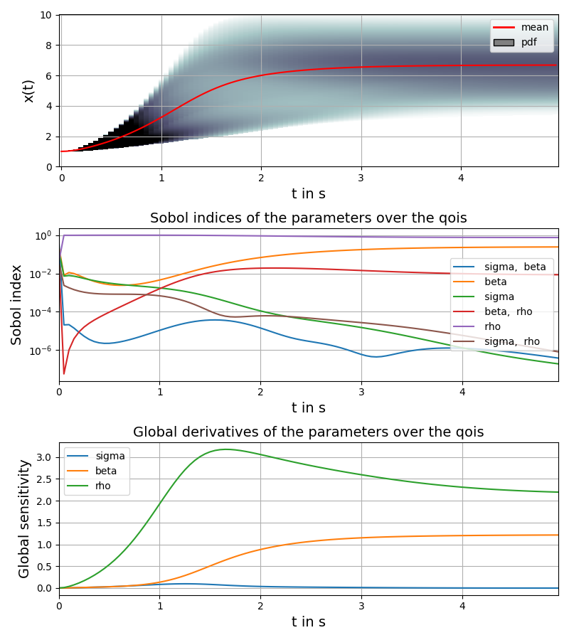
# plot time course of mean together with probability density, sobol sensitivity coefficients and global derivatives
t = np.arange(0.0, parameters["t_end"], parameters["step_size"])
pygpc.plot_sens_summary(session=session,
                        coeffs=coeffs,
                        sobol=sobol,
                        gsens=gsens,
                        plot_pdf_over_output_idx=True,
                        qois=t,
                        mean=pygpc.SGPC.get_mean(coeffs),
                        std=pygpc.SGPC.get_std(coeffs),
                        x_label="t in s",
                        y_label="x(t)",
                        zlim=[0, 0.4])

#
# On Windows subprocesses will import (i.e. execute) the main module at start.
# You need to insert an if __name__ == '__main__': guard in the main module to avoid
# creating subprocesses recursively.
#
# if __name__ == '__main__':
#     main()

> Loading gpc session object: tmp/example_lorenz.hdf5
> Loading gpc coeffs: tmp/example_lorenz.hdf5
> Adding results to: tmp/example_lorenz.hdf5