Note
Click here to download the full example code
L1 optimal sampling#
Before explaining the different types of L1 optimal grids a brief motivation for the L1-optimization and further the L1 optimal sampling that aims to strengthen the benefit from this procedure is given. L1 optimization is used for solving the following linear algebra problem at the core of the gPC for underdetermined system where the number of model evaluations is less than the number of gPC coefficients to be determined.
In this case the matrix \(\mathbf{\Psi}\) is of size \(M\times N\) and the coefficient vector \(\mathbf{C}\) of size \(N\), where \(N<M\). In other words we’re trying to fit more coefficients then we have data points. This procedure is most effective if the vector or array of coefficients has a high amount of vanishing and thus not needed entries. This type of problem can also be called sparse recovery or compressive sensing.
L1 optimal sampling seeks to tune the grid composition for solving such a problem efficiently. Most grids in this category are based on coherence optimal samples drawn from a sampling strategy introduced by Hampton and Doostan (2015) in the framework of gPC.
A variety of grid types can be build upon this idea:
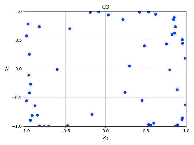
Coherence optimal sampling (CO)#
Coherence optimal sampling seeks to minimize the spectral matrix norm between the Gram matrix of the gPC matrix and the identify matrix. The Gram matrix is defined by:
and its distance from the identity matrix by:
This objective is usually sidestepped by minimizing the coherence parameter \(\mu\) instead:
where \(\xi\) are the random variables representing the input parameters, \(\Omega\) is the entirety of all random variables \(w\) are weighting functions discussed below and \(\psi_j\) are the elements of the matrix \(\mathbf{\Psi}\). The minimization can be realized by sampling the input parameters with an alternative distribution:
where \(c\) is a normalization constant, \(P(\mathbf{\xi})\) is the joint probability density function of the original input distributions and \(B(\mathbf{\xi})\) is an upper bound of the polynomial chaos basis:
To avoid defining the normalization constant $c$ a Markov Chain Monte Carlo approach using a Metropolis-Hastings sampler [2] is used to draw samples from \(P_{\mathbf{Y}}(\mathbf{\xi})\). For the Mertopolis-Hastings sampler it is necessary to define a sufficient candidate distribution. For a coherence optimal sampling this is realized by a proposal distribution \(g(\xi)\) (see the method introduced by Hampton). By sampling from a different distribution then :math:’P(xi)’ however it is not possible to guarantee \(\mathbf{\Psi}\) to be a matrix of orthonormal polynomials.
Therefore \(\mathbf{W}\) needs to be a diagonal positive-definite matrix of weight-functions \(w(\xi)\) which is then applied to:
In practice it is possible to compute \(\mathbf{W}\) with:
Example#
In order to create a coherence optimal grid of sampling points, we have to define the random parameters and create a gpc object.
import pygpc
import numpy as np
import seaborn as sns
import matplotlib.pyplot as plt
from collections import OrderedDict

# define model
model = pygpc.testfunctions.RosenbrockFunction()

# define parameters
parameters = OrderedDict()
parameters["x1"] = pygpc.Beta(pdf_shape=[1, 1], pdf_limits=[-np.pi, np.pi])
parameters["x2"] = pygpc.Beta(pdf_shape=[1, 1], pdf_limits=[-np.pi, np.pi])

# define problem
problem = pygpc.Problem(model, parameters)

# create gpc object
gpc = pygpc.Reg(problem=problem,
                order=[5]*problem.dim,
                order_max=5,
                order_max_norm=1,
                interaction_order=2,
                interaction_order_current=2,
                options=None,
                validation=None)

# create a coherence optimal grid
grid_co = pygpc.CO(parameters_random=parameters,
                   n_grid=50,
                   gpc=gpc,
                   options={"seed": None,
                            "n_warmup": 1000})

# An example of how the samples are distributed in the probability space is given below:

plt.scatter(grid_co.coords_norm[:, 0], grid_co.coords_norm[:, 1],
              color=sns.color_palette("bright", 5)[0])

plt.xlabel("$x_1$", fontsize=12)
plt.ylabel("$x_2$", fontsize=12)
plt.xticks(np.linspace(-1, 1, 5))
plt.yticks(np.linspace(-1, 1, 5))
plt.xlim([-1, 1])
plt.ylim([-1, 1])
plt.title("CO")
plt.grid()
plt.tight_layout()
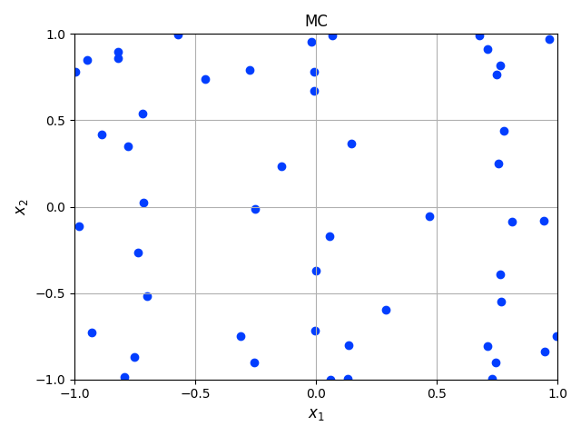
Mutual coherence optimal sampling (mc)#
The mutual coherence of a matrix measures the cross-correlations between its columns by evaluating the largest absolute and normalized inner product between different columns. It is given by:
The objective is to select sampling points to minimize \(\mu(\mathbf{\Psi})\) for a desired L1 optimal design. Minimizing the mutual-coherence considers only the worst-case scenario and does not account to improve compressive sampling performance in general.
# create a mutual coherence optimal grid
grid_mc = pygpc.L1(parameters_random=parameters,
                   n_grid=50,
                   gpc=gpc,
                   options={"criterion": ["mc"],
                            "method": "greedy",
                            "n_pool": 1000,
                            "seed": None})

# An example of how the samples are distributed in the probability space is given below:
plt.scatter(grid_mc.coords_norm[:, 0], grid_mc.coords_norm[:, 1],
              color=sns.color_palette("bright", 5)[0])

plt.xlabel("$x_1$", fontsize=12)
plt.ylabel("$x_2$", fontsize=12)
plt.xticks(np.linspace(-1, 1, 5))
plt.yticks(np.linspace(-1, 1, 5))
plt.xlim([-1, 1])
plt.ylim([-1, 1])
plt.title("MC")
plt.grid()
plt.tight_layout()
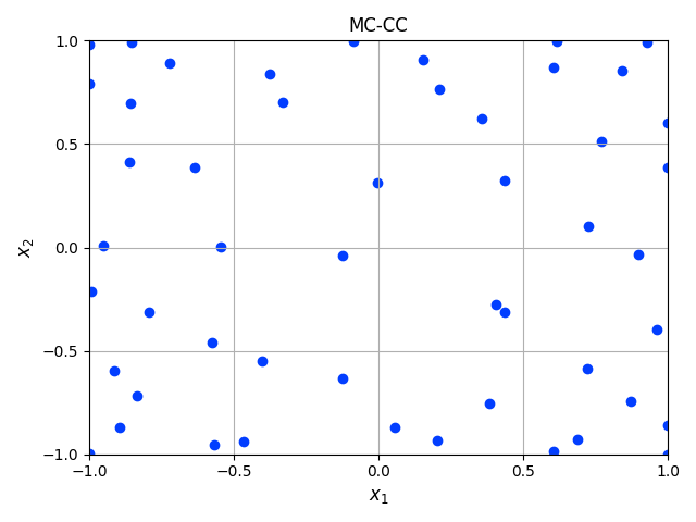
Mutual coherence and average cross-correlation optimal sampling (mc-cc)#
An improvement of sampling designs that are only optimized in the mutual coherence is done by adding the average cross- correlation as a measure for a two-fold optimization with the benefit of further robustness in its efficient sparse recovery. The average cross-correlation is defined by:
where \(||\cdot||_F\) denotes the Frobenius norm and \(N := K \times (K - 1)\) is the total number of column pairs. In this context, Alemazkoor and Meidani (2018) proposed a hybrid optimization criteria, which minimizes the average-cross correlation \(\gamma(\mathbf{\Psi})\) and the mutual coherence \(\mu(\mathbf{\Psi})\):
with \(\boldsymbol\mu = (\mu_{1}, \mu_{2}, ..., \mu_{i})\) and \(\boldsymbol\gamma = (\gamma_1, \gamma_2, ..., \gamma_i)\)
# create a mutual coherence and cross correlation optimal grid
grid_mc_cc = pygpc.L1(parameters_random=parameters,
                      n_grid=50,
                      gpc=gpc,
                      options={"criterion": ["mc", "cc"],
                               "method": "greedy",
                               "n_pool": 1000,
                               "seed": None})

# An example of how the samples are distributed in the probability space is given below:
plt.scatter(grid_mc_cc.coords_norm[:, 0], grid_mc_cc.coords_norm[:, 1],
              color=sns.color_palette("bright", 5)[0])

plt.xlabel("$x_1$", fontsize=12)
plt.ylabel("$x_2$", fontsize=12)
plt.xticks(np.linspace(-1, 1, 5))
plt.yticks(np.linspace(-1, 1, 5))
plt.xlim([-1, 1])
plt.ylim([-1, 1])
plt.title("MC-CC")
plt.grid()
plt.tight_layout()
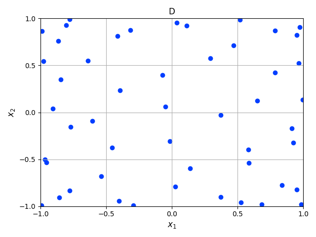
D-optimal sampling#
Further a selection of optimization criteria derived from \(\mathbf{G_\Psi}\) and the identification of corresponding optimal sampling locations is the core concept of optimal design of experiment (ODE). The most popular criterion for that is \(D\)-optimality where it the goal to increase the information content from a given amount of sampling points by minimizing the determinant of the inverse of the Gramian:
\(D\)-optimal designs are focused on precise estimation of the coefficients. Besides \(D\)-optimal designs, there exist are a lot of other alphabetic optimal designs such as \(A\)-, \(E\)-, \(I\)-, or \(V\)- optimal designs with different goals and criteria. A nice overview about them can be found by Atkinson (2007) and Pukelsheim (2006).
# create a D optimal grid
grid_d = pygpc.L1(parameters_random=parameters,
                      n_grid=50,
                      gpc=gpc,
                      options={"criterion": ["D"],
                               "method": "greedy",
                               "n_pool": 1000,
                               "seed": None})

# An example of how the samples are distributed in the probability space is given below:
plt.scatter(grid_d.coords_norm[:, 0], grid_d.coords_norm[:, 1],
              color=sns.color_palette("bright", 5)[0])

plt.xlabel("$x_1$", fontsize=12)
plt.ylabel("$x_2$", fontsize=12)
plt.xticks(np.linspace(-1, 1, 5))
plt.yticks(np.linspace(-1, 1, 5))
plt.xlim([-1, 1])
plt.ylim([-1, 1])
plt.title("D")
plt.grid()
plt.tight_layout()
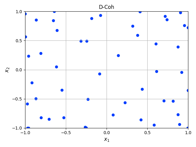
D-coherence optimal sampling#
\(D\)-optimal designs can even be combined with coherence optimal designs by using a pool of already coherence optimal samples and then applying the optimization of the \(D\) criterion on it. This has been shown to be a promising approach for special cases of functions by Diaz et al. (2017). For that and the other L1 optimal sampling schemes we used a greedy algorithm to determine the sets of sampling points. In this algorithm, we generate a pool of coherence optimal samples using the Metropolis-Hastings sampler and randomly pick an initial sample. In the next iteration we successively add a sampling point and calculate the respective optimization criteria. After evaluating all possible candidates, we add the sampling point yielding the best criterion and append it to the existing set. This is repeated until the sampling set has the desired size.
# create a D-coherence optimal grid
grid_d_coh = pygpc.L1(parameters_random=parameters,
                      n_grid=50,
                      gpc=gpc,
                      options={"criterion": ["D-coh"],
                               "method": "greedy",
                               "n_pool": 1000,
                               "seed": None})

# An example of how the samples are distributed in the probability space is given below:
plt.scatter(grid_d_coh.coords_norm[:, 0], grid_d_coh.coords_norm[:, 1],
              color=sns.color_palette("bright", 5)[0])

plt.xlabel("$x_1$", fontsize=12)
plt.ylabel("$x_2$", fontsize=12)
plt.xticks(np.linspace(-1, 1, 5))
plt.yticks(np.linspace(-1, 1, 5))
plt.xlim([-1, 1])
plt.ylim([-1, 1])
plt.title("D-Coh")
plt.grid()
plt.tight_layout()

# L1 designs with different optimization criteria can be created using the "criterion" argument in the options
# dictionary.
#
# Options
# ^^^^^^^
#
# The following options are available for L1-optimal grids:
#
# **pygpc.CO()**
#
# - seed: set a seed to reproduce the results (default: None)
# - n_warmup: the number of samples that are discarded in the Metropolis-Hastings sampler before samples are accepted (default: max(200, 2*n_grid), here n_grid is the amount of samples that are meant to be generated)
#
# **pygpc.L1()**
#
# - seed: set a seed to reproduce the results (default: None)
# - method:
#    - "greedy": greedy algorithm (default, recommended)
#    - "iter": iterative algorithm (faster but does not perform as good as "greedy")
# - criterion:
#    - ["mc"]: mutual coherence optimal
#    - ["mc", "cc"]: mutual coherence and cross correlation optimal
#    - ["D"]: D optimal
#    - ["D-coh"]: D and coherence optimal
# - n_pool: number of grid points in overall pool to select optimal points from (default: 10.000)
# - n_iter: number of iterations used for the "iter" method (default: 1000)

# The sampling method can be selected accordingly for each gPC algorithm by setting the following options
# when setting up the algorithm:
options = dict()
...
options["grid"] = pygpc.L1
options["grid_options"] = {"seed": None,
                           "method": "greedy",
                           "criterion": ["mc", "cc"],
                           "n_pool": 1000}
...

# References
# ^^^^^^^^^
# .. [1] Hampton, J., Doostan A., Coherence motivated sampling and convergence analysis of least
#     squares polynomial Chaos regression, Computer Methods in Applied Mechanics and Engineering,
#     290 (2015), 73–97.
# .. [2] Hastings, W. K., Monte Carlo sampling methods using Markov chains and their applications,
#     1970.
# .. [3] Alemazkoor N., Meidani, H., A near-optimal sampling strategy for sparse recovery of polynomial
#     chaos expansions, Journal of Computational Physics, 371 (2018), 137–151
# .. [4] Atkinson, A. C., Optimum experimental designs, with SAS, vol. 34 of Oxford statistical
#    science series, Oxford Univ. Press, Oxford, 2007, URL http://site.ebrary.com/lib/academiccompletetitles/home.action.
# .. [5] Pukelsheim, F., Optimal design of experiments, SIAM, 2006.
# .. [6] Diaz, P., Doostan, A., and Hampton, J., Sparse polynomial chaos expansions via compressed sensing
#    and D-optimal design, Computer Methods in Applied Mechanics and Engineering, 336 (2018), 640–666.

# When using Windows you need to encapsulate the code in a main function and insert an
# if __name__ == '__main__': guard in the main module to avoid creating subprocesses recursively:
#
# if __name__ == '__main__':
#     main()
Ellipsis
Total running time of the script: ( 0 minutes 9.679 seconds)