How to define a gPC problem

Random parameters

The \(d\) parameters of interest, which are assumed to underlie a distinct level of uncertainty, are modeled as a \(d\)-variate random vector denoted by \(\mathbf{\xi} = (\xi_1, \xi_2, ... \xi_d)\). It is defined in the probability space \((\Theta, \Sigma, P)\). The event or random space \(\Theta\) contains all possible events. \(\Sigma\) is a \(\sigma\)-Algebra over \(\Theta\), containing sets of events, and \(P\) is a function assigning the probabilities of occurrence to the events. The number of random variables \(d\) determines the dimension of the uncertainty problem. It is assumed that the parameters are statistically mutually independent from each other. In order to perform a gPC expansion, the random variables must have a finite variance, which defines the problem in the \(L_2\)-Hilbert space.

The probability density function (pdf) \(p_i(\xi_i)\), with \(i=1,...,d\), has to be defined for each random variable \(\xi_i\).

Currently, pygpc supports:

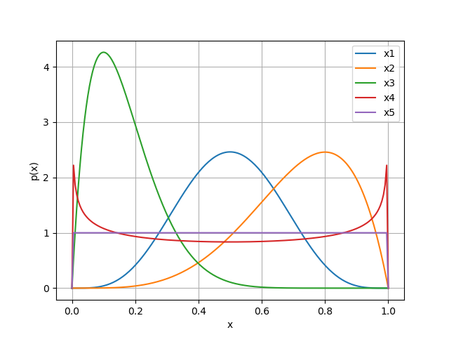
Beta distributed random variables

Probability density function:

\[p(x) = \left(\frac{\Gamma(p)\Gamma(q)}{\Gamma(p+q)}(b-a)^{(p+q-1)}\right)^{-1} (x-a)^{(p-1)} (b-x)^{(q-1)}\]

The shape parameters of beta distributed random variable are defined with the parameter pdf_shape \(=[p, q]\) and the limits with pdf_limits \(=[a, b]\).

import pygpc
from collections import OrderedDict

parameters = OrderedDict()
parameters["x1"] = pygpc.Beta(pdf_shape=[5, 5], pdf_limits=[0, 1])
parameters["x2"] = pygpc.Beta(pdf_shape=[5, 2], pdf_limits=[0, 1])
parameters["x3"] = pygpc.Beta(pdf_shape=[2, 10], pdf_limits=[0, 1])
parameters["x4"] = pygpc.Beta(pdf_shape=[0.75, 0.75], pdf_limits=[0, 1])
parameters["x5"] = pygpc.Beta(pdf_shape=[1, 1], pdf_limits=[0, 1])
ax = parameters["x1"].plot_pdf()
ax = parameters["x2"].plot_pdf()
ax = parameters["x3"].plot_pdf()
ax = parameters["x4"].plot_pdf()
ax = parameters["x5"].plot_pdf()
_ = ax.legend(["x1", "x2", "x3", "x4", "x5"])

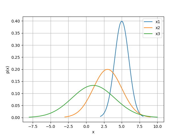
Normal distributed random variables

Probability density function:

\[p(x) = \frac{1}{\sqrt{2\pi\sigma^2}}\exp{-\frac{(x-\mu)^2}{2\sigma^2}}\]

The mean and the standard deviation are defined with the parameter pdf_shape \(=[\mu, \sigma]\).

parameters = OrderedDict()
parameters["x1"] = pygpc.Norm(pdf_shape=[5, 1])
parameters["x2"] = pygpc.Norm(pdf_shape=[3, 2])
parameters["x3"] = pygpc.Norm(pdf_shape=[1, 3])
ax = parameters["x1"].plot_pdf()
ax = parameters["x2"].plot_pdf()
ax = parameters["x3"].plot_pdf()
_ = ax.legend(["x1", "x2", "x3"])

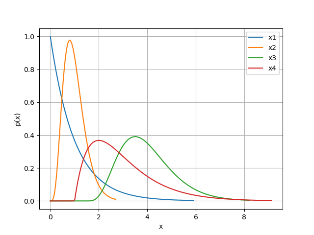
Gamma distributed random variables

Probability density function:

\[p(x) = \frac{\beta^{\alpha}}{\Gamma(\alpha)}x^{\alpha-1}e^{\beta x}\]

The shape, rate and the location of the gamma distributed random variable is defined with the parameter pdf_shape \(=[\alpha, \beta, loc]\)

parameters = OrderedDict()
parameters["x1"] = pygpc.Gamma(pdf_shape=[1, 1, 0])
parameters["x2"] = pygpc.Gamma(pdf_shape=[5, 5, 0])
parameters["x3"] = pygpc.Gamma(pdf_shape=[5, 2, 1.5])
parameters["x4"] = pygpc.Gamma(pdf_shape=[2, 1, 1])

ax = parameters["x1"].plot_pdf()
ax = parameters["x2"].plot_pdf()
ax = parameters["x3"].plot_pdf()
ax = parameters["x4"].plot_pdf()
_ = ax.legend(["x1", "x2", "x3", "x4"])

Problem definition

The gPC problem is initialized with the model and the parameters defined before:

# define model
model = pygpc.testfunctions.Peaks()

# define problem
problem = pygpc.Problem(model, parameters)