Dimensionality reduction

Introduction

A large number of models show redundancies in the form of correlations between the parameters under investigation. Especially in the case of high-dimensional problems, the correlative behavior of the target variable as a function of the parameters is usually completely unknown. Correlating parameters can be combined into surrogate parameters by means of a principal component analysis, which enables a reduction of the effective parameter number. This significantly reduces the computational effort compared to the original problem with only minor losses in modeling accuracy.

In this case, the \(n_d\) original random variables \(\mathbf{\xi}\) are reduced to a new set of \(n_d'\) random variables \(\mathbf{\eta}\), where \(n_d'<n_d\) and which are a linear combination of the original random variables such that:

\[\mathbf{\eta} = [\mathbf{W}]\mathbf{\xi}\]

The challenging part is to determine the projection matrix \([\mathbf{W}]\), which rotates the basis and reformulates the original problem to a more efficient one without affecting the solution accuracy too much. Determining the projection matrix results in a separate optimization problem besides of determining the gPC coefficients. Several approaches where investigated in the literature from for example Tipireddy and Ghanem (2014) as well as Tsilifis et al. (2019). They solved the coupled optimization problems alternately, i.e. keeping the solution of the one fixed while solving the other until some convergence criterion is satisfied.

Method

In pygpc, the projection matrix \([\mathbf{W}]\) is determined from the singular value decomposition of the gradients of the solution vector along the original parameter space. The gradients of the quantity of interest (QoI) along \(\mathbf{\xi}\) are stored in the matrix \([\mathbf{Y}_\delta]\):

\[\begin{split}[\mathbf{Y}_\partial] = \left[ \begin{array}{ccc} \left.\frac{\partial y}{\partial\xi_1}\right|_{\xi^{(1)}} & \ldots & \left.\frac{\partial y}{\partial\xi_d}\right|_{\xi^{(1)}}\\ \left.\frac{\partial y}{\partial\xi_1}\right|_{\xi^{(2)}} & \ldots & \left.\frac{\partial y}{\partial\xi_d}\right|_{\xi^{(2)}}\\ \vdots & \ddots & \vdots\\ \left.\frac{\partial y}{\partial\xi_1}\right|_{\xi^{(n_g)}} & \ldots & \left.\frac{\partial y}{\partial\xi_d}\right|_{\xi^{(n_g)}}\\ \end{array}\right]\end{split}\]

The matrix \([\mathbf{Y}_\delta]\) is of size \(n_g \times n_d\), where \(n_g\) is the number of sampling points and \(n_d\) is the number of random variables in the original parameter space. Its SVD is given by:

\[\left[\mathbf{Y}_\delta\right] = \left[\mathbf{U}\right]\left[\mathbf{\Sigma}\right]\left[\mathbf{V}^*\right]\]

The matrix \(\left[\mathbf{\Sigma}\right]\) contains the \(n_d\) singular values \(\sigma_i\) of \([\mathbf{Y}_\delta]\). The projection matrix \([\mathbf{W}]\) is determined from the right singular vectors \([\mathbf{V}^*]\) by including principal axes up to a limit where the sum of the included singular values reaches 95% of the total sum of singular values:

\[\sum_{i=1}^{n_d'} \sigma_i \leq 0.95\sum_{i=1}^{n_d} \sigma_i\]

Hence, the projection matrix \([\mathbf{W}]\) is given by the first \(n_d'\) rows of \([\mathbf{V}^*]\).

\[\begin{split}[\mathbf{V}^*] = \left[ \begin{array}{c} [\mathbf{W}] \\ [\mathbf{W}'] \end{array}\right]\end{split}\]

The advantage of the SVD approach is that the rotation is optimal in the L2 sense because the new random variables \(\eta\) are aligned with the principal axes of the solution. Moreover, the calculation of the SVD of \(\left[\mathbf{Y}_\delta\right]\) is fast. The disadvantage of the approach is however, that the gradient of the solution vector is required to determine the projection matrix \([\mathbf{W}]\). Depending on the chosen gradient calculation approach this may result in additional function evaluations. Once the gradients have been calculated, however, the gPC coefficients can be computed with higher accuracy and less additional sampling points as it is described in the Gradient enhanced gPC. Accordingly, the choice of which method to select is (as usual) highly dependent on the underlying problem and its compression capabilities.

It is noted that the projection matrix \([\mathbf{W}]\) has to be determined for each QoI separately.

The projection approach is implemented in the following algorithms:

• Algorithm: StaticProjection

• Algorithm: RegAdaptiveProjection

• Algorithm: MEStaticProjection

• Algorithm: MERegAdaptiveProjection

Example

Lets consider the following \(n_d\) dimensional testfunction:

\[y = \cos \left( 2 \pi u + a\sum_{i=1}^{n_d}\xi_i \right)\]

with \(u=0.5\) and \(a=5.0\). Without loss of generality, we assume the two-dimensional case, i.e. \(n_d=2\), for now. This function can be expressed by only one random variable \(\eta\), which is a linear combination of the original random variables \(\xi\):

\[\eta = \sum_{i=1}^{n_d}\xi_i,\]

This function is implemented in the testfunctions module of pygpc in GenzOscillatory. In the following, we will set up a static gPC with fixed order using the previously described projection approach to reduce the original dimensionality of the problem.

Setting up the problem

import pygpc
from collections import OrderedDict

# Loading the model and defining the problem
# ------------------------------------------

# Define model
model = pygpc.testfunctions.GenzOscillatory()

# Define problem
parameters = OrderedDict()
parameters["x1"] = pygpc.Beta(pdf_shape=[1., 1.], pdf_limits=[0., 1.])
parameters["x2"] = pygpc.Beta(pdf_shape=[1., 1.], pdf_limits=[0., 1.])
problem = pygpc.Problem(model, parameters)

Setting up the algorithm

# gPC options
options = dict()
options["method"] = "reg"
options["solver"] = "Moore-Penrose"
options["settings"] = None
options["interaction_order"] = 1
options["n_cpu"] = 0
options["error_type"] = "nrmsd"
options["n_samples_validation"] = 1e3
options["error_norm"] = "relative"
options["matrix_ratio"] = 2
options["qoi"] = 0
options["fn_results"] = 'tmp/staticprojection'
options["save_session_format"] = ".pkl"
options["grid"] = pygpc.Random
options["grid_options"] = {"seed": 1}
options["n_grid"] = 100

Since we have to compute the gradients of the solution anyway for the projection approach, we will make use of them also when determining the gPC coefficients. Therefore, we enable the “gradient_enhanced” gPC. For more details please see Gradient enhanced gPC.

options["gradient_enhanced"] = True

In the following we choose the method to determine the gradients. We will use a classical first order finite difference forward approximation for now.

options["gradient_calculation"] = "FD_fwd"
options["gradient_calculation_options"] = {"dx": 0.001, "distance_weight": -2}

We will use a 10th order approximation. It is noted that the model will consist of only one random variable. Including the mean (0th order coefficient) there will be 11 gPC coefficients in total.

options["order"] = [10]
options["order_max"] = 10

Now we are defining the StaticProjection algorithm to solve the given problem.

algorithm = pygpc.StaticProjection(problem=problem, options=options)

Running the gpc

# Initialize gPC Session
session = pygpc.Session(algorithm=algorithm)

# Run gPC algorithm
session, coeffs, results = session.run()

Out:

Creating initial grid (<class 'pygpc.Grid.Random'>) with n_grid=100
Determining gPC approximation for QOI #0:
=========================================
Performing 100 simulations!

It/Sub-it: 10/1 Performing simulation 001 from 100 [                                        ] 1.0%
Total function evaluation: 0.00021028518676757812 sec

It/Sub-it: 10/1 Performing simulation 001 from 200 [                                        ] 0.5%
Gradient evaluation: 0.0012793540954589844 sec
Determine gPC coefficients using 'Moore-Penrose' solver (gradient enhanced)...
-> relative nrmsd error = 0.000693256699171336

Inspecting the gpc object

The SVD of the gradients of the solution vector resulted in the following projection matrix reducing the problem from the two dimensional case to the one dimensional case:

print(f"Projection matrix [W]: {session.gpc[0].p_matrix}")

Out:

Projection matrix [W]: [[-0.70710678 -0.70710678]]

It is of size \(n_d' \times n_d\), i.e. \([1 \times 2]\) in our case. Because of the simple sum of the random variables it can be seen directly from the projection matrix that the principal axis is 45° between the original parameter axes, exactly as the SVD of the gradient of the solution predicts. As a result, the number of gPC coefficients for a 10th order gPC approximation with only one random variable is 11:

print(f"Number of gPC coefficients: {session.gpc[0].basis.n_basis}")

Out:

Number of gPC coefficients: 11

Accordingly, the gPC matrix has 11 columns, one for each gPC coefficient:

print(f"Size of gPC matrix: {session.gpc[0].gpc_matrix.shape}")

Out:

Size of gPC matrix: (100, 11)

It was mentioned previously that the one can make use of the Gradient enhanced gPC when using the projection approach. Internally, the gradients are also rotated and the gPC matrix is extended by the gPC matrix containing the derivatives:

print(f"Size of gPC matrix containing the derivatives: {session.gpc[0].gpc_matrix_gradient.shape}")

Out:

Size of gPC matrix containing the derivatives: (100, 11)

The random variables of the original and the reduced problem can be reviewed in:

print(f"Original random variables: {session.gpc[0].problem_original.parameters_random}")
print(f"Reduced random variables: {session.gpc[0].problem.parameters_random}")

Out:

Original random variables: OrderedDict([('x1', <pygpc.RandomParameter.Beta object at 0x7f685275b6a0>), ('x2', <pygpc.RandomParameter.Beta object at 0x7f685275bb50>)])
Reduced random variables: OrderedDict([('n0', <pygpc.RandomParameter.Beta object at 0x7f68526ef610>)])

Postprocessing

The post-processing works identical as in a standard gPC. The routines identify whether the problem is reduced and provide all sensitivity measures with respect to the original model parameters.

# Post-process gPC and save sensitivity coefficients in .hdf5 file
pygpc.get_sensitivities_hdf5(fn_gpc=options["fn_results"],
                             output_idx=None,
                             calc_sobol=True,
                             calc_global_sens=True,
                             calc_pdf=False,
                             algorithm="sampling",
                             n_samples=10000)

# Get summary of sensitivity coefficients
sobol, gsens = pygpc.get_sens_summary(fn_gpc=options["fn_results"],
                                      parameters_random=session.parameters_random,
                                      fn_out=None)
print(f"\nSobol indices:")
print(f"==============")
print(sobol)

print(f"\nGlobal average derivatives:")
print(f"===========================")
print(gsens)

Out:

> Loading gpc session object: tmp/staticprojection.pkl
> Loading gpc coeffs: tmp/staticprojection.hdf5
> Adding results to: tmp/staticprojection.hdf5

Sobol indices:
==============
              sobol_norm (qoi 0)
['x1', 'x2']            0.855755
['x2']                  0.076095
['x1']                  0.075139

Global average derivatives:
===========================
    global_sens (qoi 0)
x1            -0.151716
x2            -0.151716

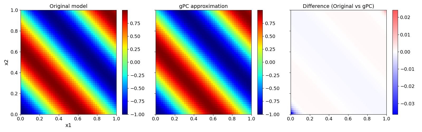
Validation

Validate gPC vs original model function (2D-surface)

The possibility of parameter reduction becomes best clear if one visualizes the function values in the parameter space. In this simple example there is almost no difference between the original model (left) and the reduced gPC (center).

pygpc.validate_gpc_plot(session=session,
                        coeffs=coeffs,
                        random_vars=list(problem.parameters_random.keys()),
                        n_grid=[51, 51],
                        output_idx=[0],
                        fn_out=None,
                        folder=None,
                        n_cpu=session.n_cpu)

References

[1]

Tipireddy, R., & Ghanem, R. (2014). Basis adaptation in homogeneous chaos spaces. Journal of Computational Physics, 259, 304-317.

[2]

Tsilifis, P., Huan, X., Safta, C., Sargsyan, K., Lacaze, G., Oefelein, J. C., Najm, H. N., & Ghanem, R. G. (2019). Compressive sensing adaptation for polynomial chaos expansions. Journal of Computational Physics, 380, 29-47.