Note
Click here to download the full example code
Setting up a custom model#
In order to analyze a mathematical model or function with pygpc, it has to be converted into a format understandable for pygpc. For this, we implemented the AbstractModel class in pygpc. You can find an example template in /templates/MyModel.py
import numpy as np
import inspect
from pygpc.AbstractModel import AbstractModel


class MyModel(AbstractModel):
    """
    MyModel evaluates something. The parameters of the model (constants and random parameters) are stored in the
    dictionary p. Their type is defined during the problem definition.

    Parameters
    ----------
    p["x1"] : float or ndarray of float [n_grid]
        Parameter 1
    p["x2"] : float or ndarray of float [n_grid]
        Parameter 2
    p["x3"] : float or ndarray of float [n_grid]
        Parameter 3

    Returns
    -------
    y : ndarray of float [n_grid x n_out]
        Results of the n_out quantities of interest the gPC is conducted for
    additional_data : dict or list of dict [n_grid]
        Additional data, will be saved under its keys in the .hdf5 file during gPC simulations.
        If multiple grid-points are evaluated in one function call, return a dict for every grid-point in a list
    """

    def __init__(self, fname_matlab=None, matlab_model=False):
        super(type(self), self).__init__(matlab_model=matlab_model)
        self.fname = inspect.getfile(inspect.currentframe())
        self.fname_matlab = fname_matlab

    def validate(self):
        pass

    def simulate(self, process_id=None, matlab_engine=None):

        y = self.p["x1"] * self.p["x2"] * self.p["x3"]
        y = y[:, np.newaxis]

        additional_data = [{"additional_data/info_1": [1, 2, 3],
                            "additional_data/info_2": ["some additional information"]}]
        additional_data = y.shape[0] * additional_data

        return y, additional_data
The actual computations are taking place in the method simulate. In this example, we simply multiply the parameters x1, x2 and x3 and return the output. During gPC, multiple simulations have to be performed for some parameter combinations. For every sampling point, pygpc initializes a new model instance and passes a dictionary p containing the parameter names together with their values in this model run. This dictionary is stored in the model (self) and can be accessed with the same parameter names defined during the problem definition (self.p[“variable_name”]).
In some cases your model may generate additional data alongside your quantity of interest (QOI). You can store this data for later use in the dictionary additional_data. This data will be saved for every sampling point in the resulting .hdf5 file.
At the end, the QOI is returned together with the additional data.
Testing the model#
# Windows users have to encapsulate the code into a main function to avoid multiprocessing errors.
# def main():
import pygpc
import numpy as np
from collections import OrderedDict
import matplotlib.pyplot as plt
# initializing the model
model = MyModel()
# initializing the problem with 2 uniform distributed random parameters
parameters = OrderedDict()
parameters["x1"] = pygpc.Beta(pdf_shape=[1, 1], pdf_limits=[-1, 1])
parameters["x2"] = pygpc.Beta(pdf_shape=[1, 1], pdf_limits=[-1, 1])
parameters["x3"] = 1.
problem = pygpc.Problem(model=model, parameters=parameters)
# generating a 100x100 2D tensored grid
x1_arr = np.linspace(-1, 1, 100)
x2_arr = np.linspace(-1, 1, 100)
x1, x2 = np.meshgrid(x1_arr, x2_arr)
# flattening the grid to [(100*100) x 2] (random parameters only)
sampling_points = np.hstack((x1.flatten()[:, np.newaxis],
x2.flatten()[:, np.newaxis]))
# initializing Computation class
# n_cpu = 0 : use this if the model is capable of to evaluate all sampling points in parallel
# n_cpu = 1 : the model is called in serial for every sampling point.
# n_cpu > 1 : A multiprocessing.Pool will be opened and n_cpu sampling points are calculated in parallel
com = pygpc.Computation(n_cpu=0)
# running the model
res = com.run(model=model,
problem=problem,
coords=sampling_points,
coords_norm=sampling_points,
i_iter=None,
i_subiter=None,
fn_results=None,
print_func_time=None)
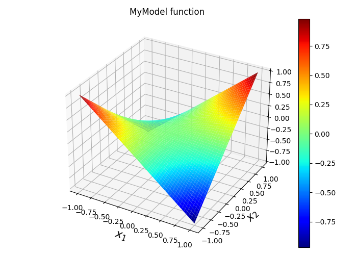
# plotting results
fig = plt.figure(figsize=(7, 5))
ax = fig.add_subplot(1, 1, 1, projection='3d')
im = ax.plot_surface(x1, x2,
np.reshape(res[:, 0], (x2_arr.size, x1_arr.size), order='c'),
cmap="jet")
ax.set_ylabel(r"$x_2$", fontsize=16)
ax.set_xlabel(r"$x_1$", fontsize=16)
fig.colorbar(im, ax=ax, orientation='vertical')
ax.set_title("MyModel function")
plt.tight_layout()
# On Windows subprocesses will import (i.e. execute) the main module at start.
# You need to insert an if __name__ == '__main__': guard in the main module to avoid
# creating subprocesses recursively.
#
# if __name__ == '__main__':
# main()
Total running time of the script: ( 0 minutes 0.433 seconds)