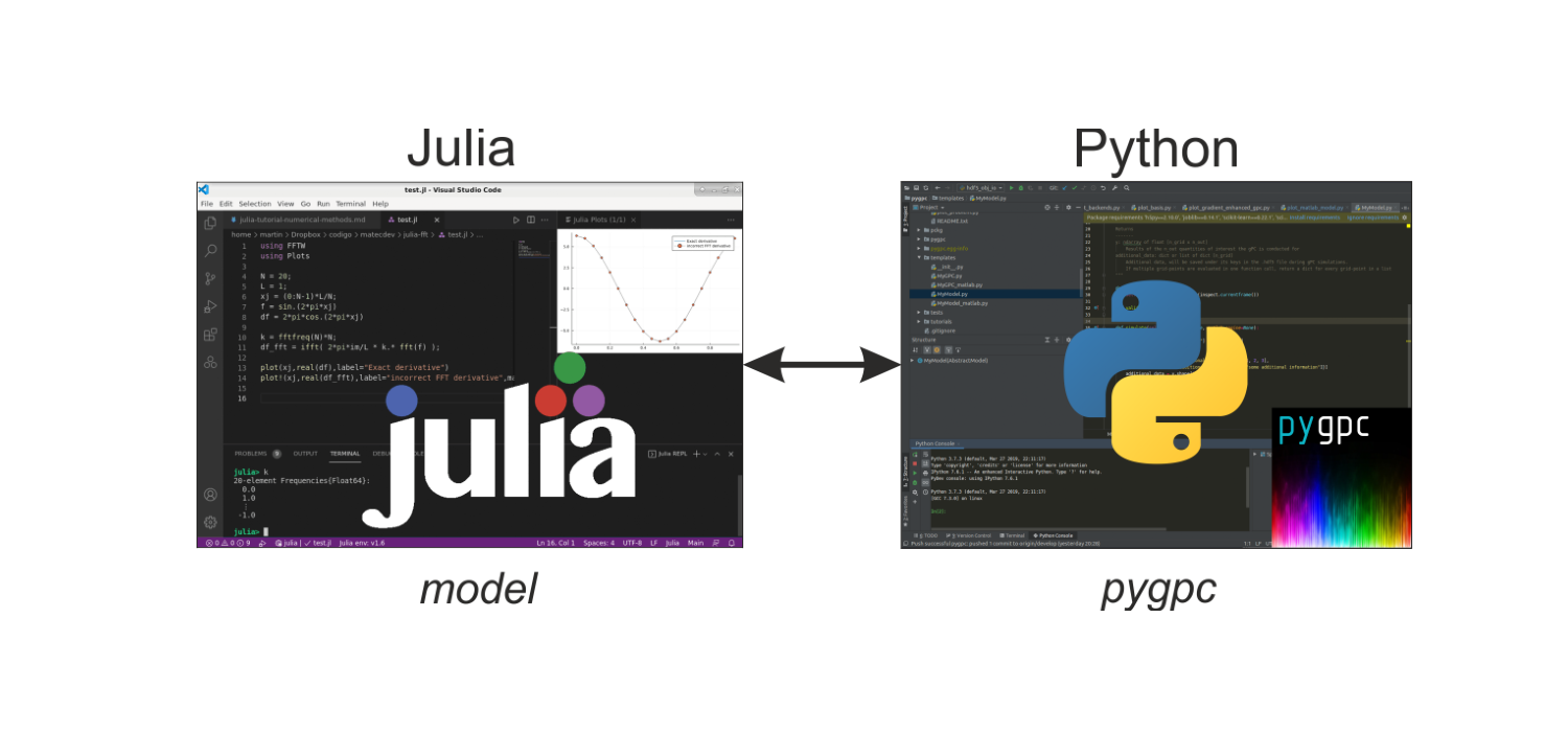
Analyzing Julia models with pygpc

You can easily analyze your models written in Julia with pygpc. In order to do so, you have to install the Julia API for Python.

import matplotlib.pyplot as plt

_ = plt.figure(figsize=[15, 7])
_ = plt.imshow(plt.imread("../images/python_julia_interface.png"))
_ = plt.axis('off')

Install Julia API for Python

If not already done, install Julia (https://julialang.org) and Python (https://www.python.org/). After installation is finished, the dependency PyCall needs to be installed in Julia. Open Julia and enter the following:

Withing Julia

import Pkg
Pkg.install("PyCall")

In Python you need to download and install the Julia package from pip for example:

pip install julia

Then open Python and install the Julia dependency (this should work if PyCall was installed beforehand):

Withing Python

import julia
julia.install()

After installation is finished, you can set:

options["julia_model"] = True

in the gPC options section of your gPC run-file.

Setting up the Julia model

Setting up the model in Julia is straight forward. You simply have to define your model as a julia function within an .jl file. In the following, you see an example model .jl file:

# Three-dimensional test function of Ishigami
function Ishigami(x1, x2, x3, a, b)
return sin.(x1) .- a .* sin.(x1).^2 .+ b .* x3.^4 .* sin.(x1)
end

If the Julia model requires the usage of Julia libraries a Julia environment needs to be created and loaded during the call from python. The environment can be created inside Julia where libraries can be installed afterwards.

import Pkg
Pkg.activate(" directory of .jl file / folder name of environment ")
Pkg.install(" library name ")

Accessing the model within pypgc

In order to call the Julia function within pygpc, we have to set up a corresponding python model as shown below. During initialization we pass the function name fname_julia, which tells pygpc where to find the model .jl function. During computation, pygpc accesses the Julia function.

The example shown below can be found in the templates folder of pygpc (/templates/MyModel_julia.py). In particular, you can find an example model-file in .../templates/MyModel_julia.py and the associated gPC run-file in .../templates/MyGPC_julia.py.

A detailed example is given in Example: Lorenz system of differential equations (Julia).

import inspect
import numpy as np
from julia import Main
from pygpc.AbstractModel import AbstractModel


class MyModel_julia(AbstractModel):
    """
    MyModel evaluates something by loading a Julia file that contains a function. The parameters
    of the model (constants and random parameters) are stored in the dictionary p. Their type is
    defined during the problem definition.

    Parameters
    ----------
    fname_julia : str
        Filename of julia function
    p["x1"] : float or ndarray of float [n_grid]
        Parameter 1
    p["x2"] : float or ndarray of float [n_grid]
        Parameter 2
    p["x3"] : float or ndarray of float [n_grid]
        Parameter 3
    p["a"] : float
        shape parameter (a=7)
    p["b"] : float
        shape parameter (b=0.1)

    Returns
    -------
    y : ndarray of float [n_grid x n_out]
        Results of the n_out quantities of interest the gPC is conducted for
    additional_data : dict or list of dict [n_grid]
        Additional data, will be saved under its keys in the .hdf5 file during gPC simulations.
        If multiple grid-points are evaluated in one function call, return a dict for every
        grid-point in a list
    """

    def __init__(self, fname_julia=None):
        if fname_julia is not None:
            self.fname_julia = fname_julia                          # filename of julia function
        self.fname = inspect.getfile(inspect.currentframe())        # filename of python function

    def validate(self):
        pass

    def simulate(self, process_id=None, matlab_engine=None):

        x1 = self.p["x1"]
        x2 = self.p["x2"]
        x3 = self.p["x3"]
        a = self.p["a"]
        b = self.p["b"]

        # access .jl file
        Main.fname_julia = self.fname_julia
        Main.include(Main.fname_julia)

        # call Julia function
        y = Main.Ishigami(x1, x2, x3, a, b)

        if y.ndim == 0:
            y = np.array([[y]])
        elif y.ndim == 1:
            y = y[:, np.newaxis]

        return y

To enable libraries via an existing environment folder as described above use Main.eval('import Pkg') and Main.eval('Pkg.activate(" folder name of environment ")') before including the .jl file. If the environment folder is not in the same place as the .jl file the complete path is needed for this call as well.

Performance Tip

You can easily vectorize basic Julia operations like (+, -, etc.) by appending a dot before them: .+, .-, etc. as shown in the function above. This can even be extended to entire functions by appending the dot after it: y = function_name(args).. With that the function should be able to process arrays for the input parameters passed in the dictionary p. And if that is the case you can set the algorithm option:

options = dict()

# ...
options["n_cpu"] = 0
# ...

To enable parallel processing in pygpc. In this way, multiple sampling points are passed to the function and processed in parallel, which speeds up your gPC analysis. A more detailed description about the parallel processing capabilities of pygpc is given in this example.