Note
Click here to download the full example code
Gradient enhanced gPC#
Introduction#
It is possible to accelerate the identification of the gPC coefficients by using the derivative information of the transfer function. The gPC matrix consists of continuously differentiable polynomials and can be extended by its partial derivatives at each sampling point. This extends the resulting system of equations to:
where the gradient gPC matrix \([\mathbf{\Psi}_\partial]\) is of size \([d N_g \times N_c]\) and contains the partial derivatives of the basis functions at each sampling point:
The solution on the right hand side is extended accordingly:
The complete system now reads:
This gradient based formulation consists of \((d+1) N_g\) equations that match both function values and gradients, in comparison to traditional approaches which consists of only \(N_g\) equations that match function values. Despite the extra computational cost required to obtain the gradients, the use of gradients improves the gPC. However, there exist several methods to determine the gradients. In the following, the implemented methods in pygpc are presented and compared.
Gradient estimation of sparse irregular datasets#
Surface interpolation finds application in many aspects of science and technology. A typical application in geological science and environmental engineering is to contour surfaces from hydraulic head measurements from irregular spaced data.
Computing gradients efficiently and accurately from sparse irregular high-dimensional datasets is challenging. The additional calculation effort should be kept as low as possible, especially in the case of computationally expensive models
Finite difference approach using forward approximation#
Let \(f:D \subset \mathbb{R}^d \rightarrow \mathbb{R}\) be differentiable at \(\mathbf{x}_0 \in D\). Taylor’s theorem for several variables states that:
where the remainder \(R_r\) has the Lagrange form:
Truncating the Taylor series after the first term leads to:
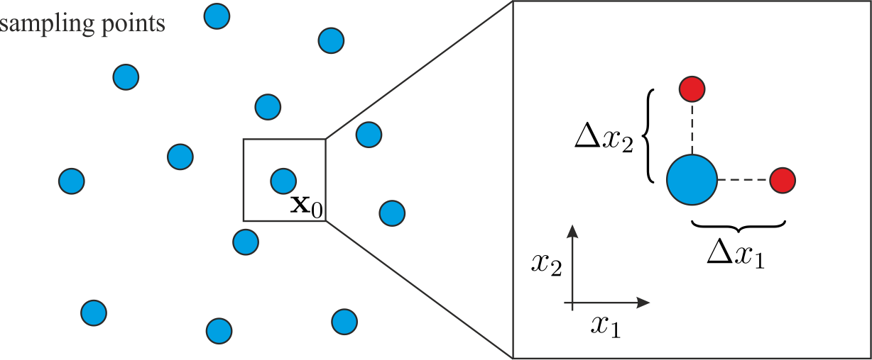
In order to approximate the gradient it is necessary to determine addtitional function values \(f(\mathbf{x}_0 + \mathbf{h})\) at small displacements \(\mathbf{h}\) in every dimension. Each additional row in the gradient gPC matrix \([\mathbf{\Psi}_\partial]\) thus requires one additional model evaluation.
This torpedoes the previously mentioned advantage of the gradient enhanced gPC approach in terms of efficacy.
Finite difference regression approach of 1st order accuracy#
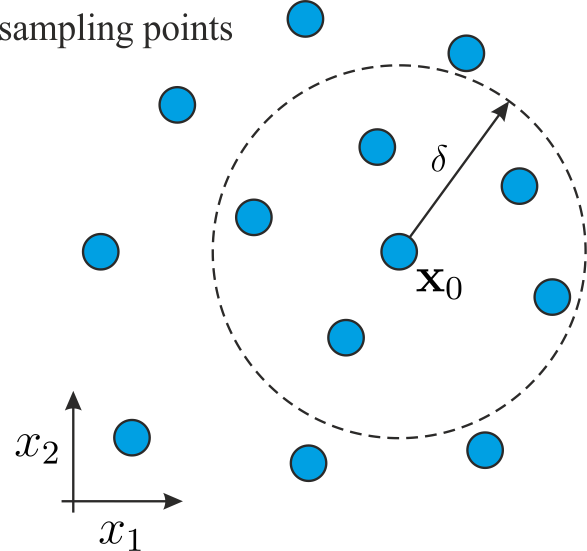
Suppose that \(\mathbf{x}_0=(x_1, ..., x_d)^\mathrm{T}\) is the point where we want to estimate the gradient and we are given \(p\) scattered data points \(\mathbf{x}_i = (x_{1,i}, ..., x_{d,i}), i = 1, ..., p\), which are located closely to \(\mathbf{x}_0\) such that \(\mathbf{x}_i \in \mathcal{B}_\delta(\mathbf{x}_0)\).
Truncating the Taylor expansion after the first term allows to write an overdetermined system of equations for \(\mathbf{g}=\left(\frac{\partial f}{\partial x_1}, ... , \frac{\partial f}{\partial x_d} \right)^\mathrm{T}\) in the form:
whose least squares solution provides a first order estimate of the gradient. The matrix \(\mathbf{D}\in\mathbb{R}^{p \times d}\) contains the distances between the surrounding points \(\mathbf{x}_i\) and the point \(\mathbf{x}_0\) and is given by:
The differences of the model solutions \(\delta f_i = f(\mathbf{x}_0 + \delta\mathbf{x}_i)-f(\mathbf{x}_0)\) are collected in the vector \(\delta \mathbf{f} \in \mathbb{R}^{p \times 1}\).
Each adjacent point may be weighted by its distance to \(\mathbf{x}_0\). This can be done by introducing a weight matrix \([\mathbf{W}] = \mathrm{diag}(\left\lvert\delta\mathbf{x}_1\right\lvert^{\alpha}, ..., \left\lvert\delta\mathbf{x}_p\right\lvert^{\alpha})\) with \(\alpha=-1\) for inverse distance or \(\alpha=-2\) for inverse distance squared.
The least squares solution of the gradient is then given by:
This procedure has to be repeated for every sampling point \(\mathbf{x}_0\). With this approach, it is possible to estimate the gradients only from the available data points without the need to run additional simulations. However, one has to suitably choose the values of \(\delta\) and \(\alpha\). If the sampling points are too far away from each other, it may not be possible to estimate the gradient accurately.
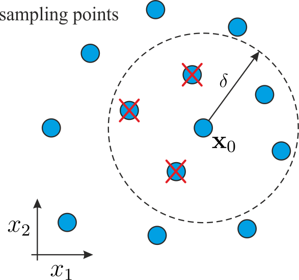
Finite difference regression approach of 2nd order accuracy#
Truncating the Taylor expansion after the second term enables the following overdetermined system to be solved, in the least squared sense, to obtain a second order approximation for the gradient:
where the second order distance matrix \([\mathbf{M}] \in \mathbb{R}^{p \times \sum_{i=1}^{d} i}\) given by:
The vector \(\mathbf{z}=\left(\frac{\partial^2 f}{\partial x_1^2}, \frac{\partial^2 f}{\partial x_1 x_2} , ..., \frac{\partial^2 f}{\partial x_d^2}\right)^\mathrm{T}\) contains the second derivatives. The new system of equations can be written as:
Applying the weight matrix \([\mathbf{W}] = \mathrm{diag}(\left\lvert\delta\mathbf{x}_1 \right\lvert^{\alpha}, ..., \left\lvert\delta\mathbf{x}_p\right\lvert^{\alpha})\) leads:
from which it can be seen that a more accurate estimate of the gradient than that offered as the previous approach can be obtained if the second order derivative terms are eliminated from the system. This elimination can be performed using QR decomposition of \([\mathbf{W}][\mathbf{M}]\), namely \([\mathbf{Q}]^{\mathrm{T}}[\mathbf{W}][\mathbf{M}] = [\mathbf{T}]\) with \([\mathbf{Q}]^{\mathrm{T}} \in \mathbb{R}^{p \times p}\) and \([\mathbf{T}]\in \mathbb{R}^{p \times \sum_{i=1}^{d} i}\), which has upper trapezoidal form. Applying \([\mathbf{Q}]^{\mathrm{T}}\) to the system of equations leads:
Because \([\mathbf{T}]\) is of upper trapezoidal form, one can eliminate the influence of the second order derivatives in \(\mathbf{z}\) by discarding the first \(\sum_{i=1}^{d} i\) equations. The least square solution of the remaining \(p-\sum_{i=1}^{d} i\) equations then provides a second order accurate estimate of the gradient \(\mathbf{g}\).
This approach is more accurate than the first order approximation but needs more sampling points because of reduction of the system.
Although the initial thought might be that the ordering of the equations would have some impact on the gradient estimation process, this is indeed not the case. To see why, let \([\mathbf{R}] \in \mathbb{R}^{p \times p}\) be a perturbation matrix that permutes the rows of \([\mathbf{W}][\mathbf{M}]\). Because the orthogonal reduction of \([\mathbf{W}][\mathbf{M}]\) produces unique matrices \([\mathbf{Q}]\) and \([\mathbf{T}]\) such that \([\mathbf{Q}]^{\mathrm{T}}[\mathbf{W}][\mathbf{M}] = [\mathbf{T}]\) it follows that applying orthogonal reduction to the permuted system \([\mathbf{R}][\mathbf{W}][\mathbf{M}]\mathbf{x} = \delta \mathbf{f}\) yields with \([\tilde{\mathbf{Q}}]^{\mathrm{T}}[\mathbf{R}][\mathbf{W}][\mathbf{M}] = [\mathbf{T}]\) and \([\mathbf{Q}] = [\mathbf{R}]^\mathrm{T}[\tilde{\mathbf{Q}}]\) exactly the same system as before.
# Comparison between the gradient estimation techniques
# ^^^^^^^^^^^^^^^^^^^^^^^^^^^^^^^^^^^^^^^^^^^^^^^^^^^^^

# Windows users have to encapsulate the code into a main function to avoid multiprocessing errors.
# def main():

import pygpc
from collections import OrderedDict
import matplotlib.pyplot as plt
from matplotlib.patches import Circle
import pandas as pd
import numpy as np
import seaborn as sns
We are going to compare the forward approximation method (most exact but needs additional simulations) with the first and second order approximations. For each method, we define different distances/radii \(dx\):
methods = ["FD_fwd", "FD_1st", "FD_2nd"]
dx = [1e-3, 0.1, 0.2]
We are going to compare the methods using the “Peaks” function and we are defining the parameter space by setting up the problem:
# define model
model = pygpc.testfunctions.Peaks()

# define problem
parameters = OrderedDict()
parameters["x1"] = pygpc.Beta(pdf_shape=[1, 1], pdf_limits=[1.2, 2])
parameters["x2"] = 1.
parameters["x3"] = pygpc.Beta(pdf_shape=[1, 1], pdf_limits=[0, 0.6])
problem = pygpc.Problem(model, parameters)
Depending on the grid and its density, the methods will behave differently. Here, we use 100 random sampling points in the parameter space defined before.
# define grid
n_grid = 100
grid = pygpc.Random(parameters_random=problem.parameters_random,
                    n_grid=n_grid,
                    options={"seed": 1})
We are setting up a Computation instance to evaluate the model function in the 100 grid points
# initializing Computation class
com = pygpc.Computation(n_cpu=0, matlab_model=False)

# evaluating model function
res = com.run(model=model,
              problem=problem,
              coords=grid.coords,
              coords_norm=grid.coords_norm,
              i_iter=None,
              i_subiter=None,
              fn_results=None,
              print_func_time=False)
We are looping over the different methods and evaluate the gradients. The forward approximation method “FD_fwd” returns the gradient for every grid point whereas the first and second order approximation “FD_1st” and “FD_2nd” only return the gradient in grid points if they have sufficient number of neighboring points within radius \(dx\). The indices stored in “gradient_idx” are the indices of the grid points where the gradients are computed.
df = pd.DataFrame(columns=["method", "nrmsd", "coverage"])
grad_res = dict()
gradient_idx = dict()

# determine gradient with different methods
for i_m, m in enumerate(methods):
    # [n_grid x n_out x dim]
    grad_res[m], gradient_idx[m] = pygpc.get_gradient(model=model,
                                                      problem=problem,
                                                      grid=grid,
                                                      results=res,
                                                      com=com,
                                                      method=m,
                                                      gradient_results_present=None,
                                                      gradient_idx_skip=None,
                                                      i_iter=None,
                                                      i_subiter=None,
                                                      print_func_time=False,
                                                      dx=dx[i_m],
                                                      distance_weight=-2)

    if m != "FD_fwd":
        df.loc[i_m, "method"] = m
        if grad_res[m] is not None:
            df.loc[i_m, "coverage"] = grad_res[m].shape[0]/n_grid
            df.loc[i_m, "nrmsd"] = pygpc.nrmsd(grad_res[m][:, 0, :], grad_res["FD_fwd"][gradient_idx[m], 0, :])
        else:
            df.loc[i_m, "coverage"] = 0
            df.loc[i_m, "nrmsd"] = None
Plotting the results#
# plot results
fig1, ax1 = plt.subplots(nrows=1, ncols=1, squeeze=True, figsize=(7.5, 5))

n_x = 250
x1, x2 = np.meshgrid(np.linspace(-1, 1, n_x), np.linspace(-1, 1, n_x))
x1x2_norm = np.hstack((x1.flatten()[:, np.newaxis], x2.flatten()[:, np.newaxis]))
x1x2 = grid.get_denormalized_coordinates(x1x2_norm)

res = com.run(model=model,
              problem=problem,
              coords=x1x2,
              coords_norm=x1x2_norm,
              i_iter=None,
              i_subiter=None,
              fn_results=None,
              print_func_time=False)

im = ax1.pcolor(x1, x2, np.reshape(res, (n_x, n_x), order='c'), cmap="jet")

ax1.scatter(grid.coords_norm[:, 0], grid.coords_norm[:, 1], s=1, c="k")

for i_m, m in enumerate(methods):
    if m != "FD_fwd" and gradient_idx[m] is not None:
        ax1.scatter(grid.coords_norm[gradient_idx[m], 0],
                    grid.coords_norm[gradient_idx[m], 1],
                    s=40, edgecolors="w",
                    color=sns.color_palette("muted", len(methods)-1)[i_m-1])

ax1.legend(["model function"] + methods, loc='upper left', bbox_to_anchor=(1, 1)) #,

for i_m, m in enumerate(methods):
    if m != "FD_fwd" and gradient_idx[m] is not None:

        for i in gradient_idx[m]:
            circ = Circle((grid.coords_norm[i, 0],
                           grid.coords_norm[i, 1]),
                          dx[i_m],
                          linestyle="--",
                          linewidth=1.2,
                          color="w", fill=True, alpha=.1)
            ax1.add_patch(circ)
            circ = Circle((grid.coords_norm[i, 0],
                           grid.coords_norm[i, 1]),
                          dx[i_m],
                          linestyle="--",
                          linewidth=1.2,
                          edgecolor=sns.color_palette("muted", len(methods)-1)[i_m-1], fill=False,alpha=1)
            ax1.add_patch(circ)

ax1.set_xlabel('$x_1$', fontsize=16)
ax1.set_ylabel('$x_2$', fontsize=16)
ax1.set_xlim([-1, 1])
ax1.set_ylim([-1, 1])
ax1.set_aspect(1.0)
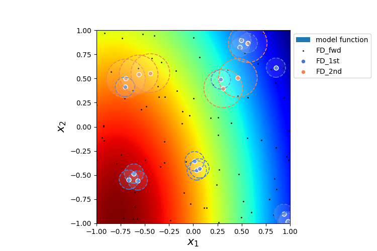
Comparing the normalized root mean square deviation of the first and second order approximation methods with respect to the forward approximation it can be seen that the 2nd order approximation is more exact. However, less points could be estimated because of the necessity to eliminate the first 3 equations. This is reflected in the lower coverage
# show summary
print(df)


# On Windows subprocesses will import (i.e. execute) the main module at start.
# You need to insert an if __name__ == '__main__': guard in the main module to avoid
# creating subprocesses recursively.
#
# if __name__ == '__main__':
#     main()
Out:
   method  ... coverage
1  FD_1st  ...     0.15
2  FD_2nd  ...     0.06

[2 rows x 3 columns]
Total running time of the script: ( 0 minutes 0.609 seconds)