Comparison of sampling schemes

For evaluating the efficiency of the sampling schemes in pygpc we compared L1 optimal sampling schemes, LHS sampling schemes and random sampling. The analysis was performed in the context of L1 minimization using the least-angle regression algorithm to fit the gPC regression models (using the LARS-solver from scipy). The sampling schemes were investigated by evaluating the quality of the constructed surrogate models considering distinct test cases representing different problem classes covering low, medium and high dimensional problems as well as on an application example to estimate the sensitivity of the self-impedance of a probe, which is used to measure the impedance of biological tissues at different frequencies. Due to the random nature, we compared the sampling schemes using statistical stability measures and evaluated the success rates to construct a surrogate model with an accuracy of < 0.1%. We observed strong differences in the convergence properties of the methods between the analyzed test functions. One of the test cases was the Ishigami function, where the results are reported in the following.

Benchmark on the Ishigami function

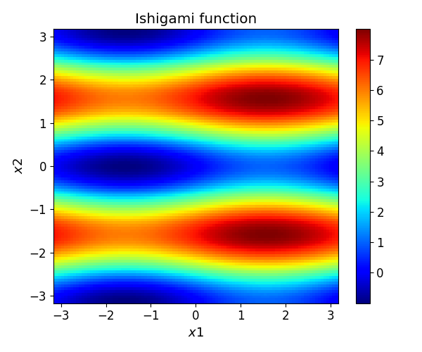
One of the testcases for different grids was the Ishigami function, which is already implemented in pygpc.

import numpy as np
from pygpc.testfunctions import plot_testfunction as plot
from collections import OrderedDict

parameters = OrderedDict()
parameters["x1"] = np.linspace(-np.pi, np.pi, 100)
parameters["x2"] = np.linspace(-np.pi, np.pi, 100)

constants = OrderedDict()
constants["a"] = 7.0
constants["b"] = 0.1
constants["x3"] = 0.0

plot("Ishigami", parameters, constants, plot_3d=False)

Because of their random nature, we compared the grid repeatedly by using N=30 repetition. For every grid instance and sampling number we recorded the normalized root mean squared deviation (NRMSD) (first row), the mean (second row) and standard deviation (third row) of the gPC approximations compared to the original model.

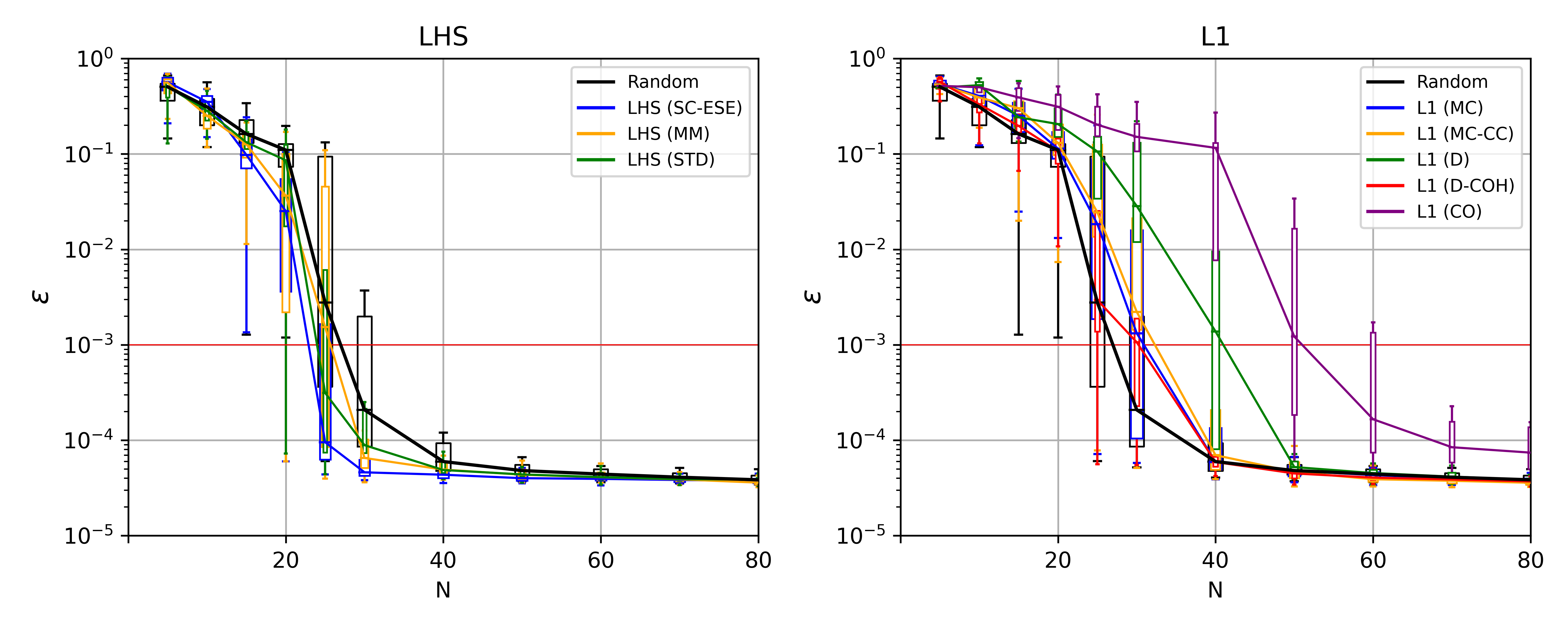
In this figure the sampling designs are abbreviated as follows:

• STD - standard LHS sampling

• MM - maximin LHS sampling

• SC-ESE - LHS sampling using enhanced stochastic evolutionary algorithm

• MC - mutual coherence optimal L1 sampling

• MC-CC - mutual coherence and average cross correlation optimal L1 sampling

• CO - coherence optimal L1 sampling

• D - \(D\) optimal sampling

• D-COH - \(D\) and coherence optimal sampling

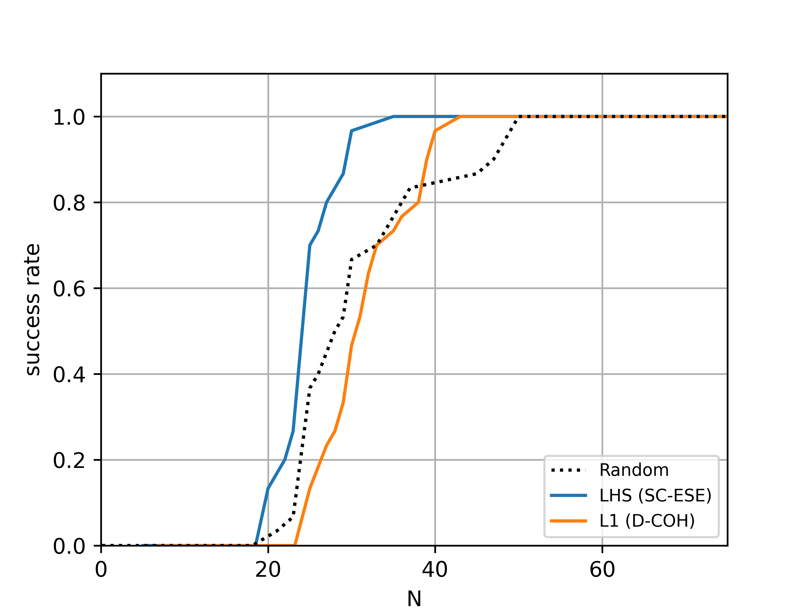
Further the success rate of the best converging grids (from all LHS and from all L1 grids) for error thresholds of 0.1%, 1%, and 10% can be seen in the following figure.

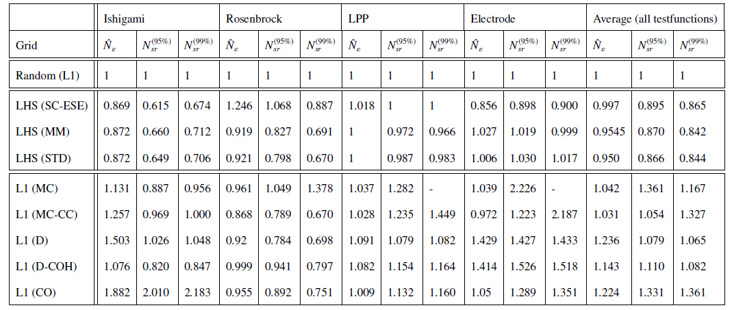
We evaluated the relative performance of the sampling schemes with respect to standard random sampling over four test cases. The Ishigami and the Rosenbrock function serve as well known test cases and the LPP (Linear-Paired-Product) function is a high dimensional test function with 30 random variables. The Electrode impedance model is a practical example. In the following table the relative and the average number of grid points \(\hat{N}_{\varepsilon}\) of the different sampling schemes to reach an NRMSD of 10−3 with respect to standard random sampling is shown. The columns for \(N_{sr}^{(95\%)}\) and \(N_{sr}^{(99\%)}\) show the number of samples needed to reach a success rate of 95% and 99% respectively.

More details about the comparison can be found in [1].

References

[1]

Weise, K., Müller, E., Poßner, L., Knösche, T. R., Comparison of the performance and reliability between improved sampling strategies for polynomial chaos expansion, AIMS Mathematical Biosciences and Engineering, 2022.