Note
Click here to download the full example code
Example: Modelling of an electrode#
About the model#
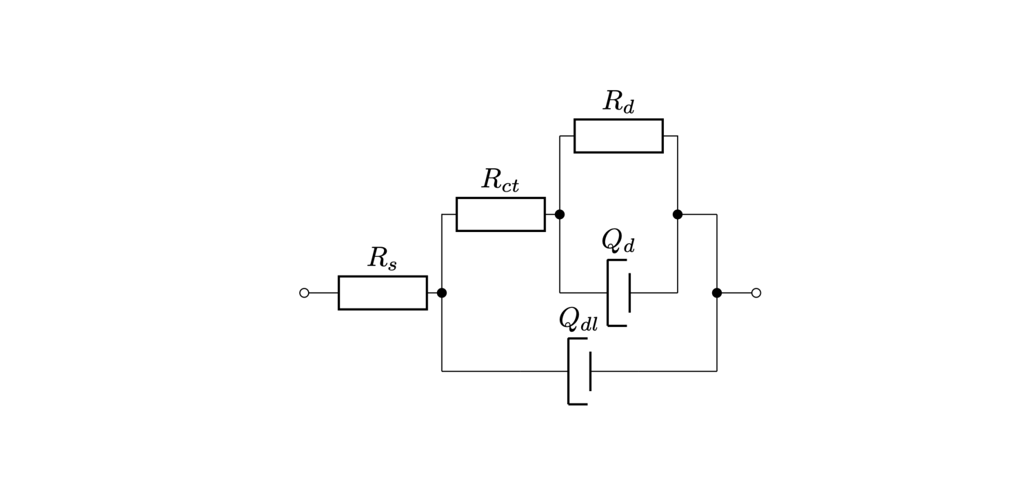
This tutorial shows the application of pygpc to an equivalent electrical circuit, modelling the impedance of an open-ended coaxial electrode. The model consists of a Randles circuit that was modified according to the coaxial geometry of the electrode. The parameters model the different contributions of the physical phenomena as follows:
\(R_d\) models the contribution of the serial resistance of an electrolyte that the electrode is dipped into.
\(Q_{dl}\) models the distributed double layer capacitance of the electrode.
\(R_{ct}\) models the charge transfer resistance between the electrode and the electrolyte
\(Q_d\) and \(R_d\) model the diffusion of charge carriers and other particles towards the electrode surface.
The elements \(Q_{dl}\) and \(Q_d\) can be described with: \(\frac{1}{Q(j\omega)^\alpha}\) The equation depends on the angular frequency \(\omega\) as a variable and \(Q\) and \(\alpha\) as parameters.
The impedance of the equivalent circuit is complex valued, has seven parameters \(R_s\), \(R_{ct}\), \(R_d\), \(Q_d\), \(\alpha_d\), \(Q_{dl}\), \(\alpha_{dl}\) and one variable \(\omega\).
The model returns an array of containing the real and imaginary part of every frequency point. Every element of this array is a quantity of interest (QoI) and a gPC is computed for every quantity of interest.
# Windows users have to encapsulate the code into a main function to avoid multiprocessing errors.
# def main():
import matplotlib.pyplot as plt

_ = plt.figure(figsize=[15, 7])
_ = plt.imshow(plt.imread("../images/modified_Randles_circuit.png"))
_ = plt.axis('off')
Loading the model and defining the problem#
import pygpc
import numpy as np
from collections import OrderedDict

fn_results = 'GPC/electrode'   # filename of output
save_session_format = ".hdf5"  # file format of saved gpc session ".hdf5" (slow) or ".pkl" (fast)

# define model
model = pygpc.testfunctions.ElectrodeModel()

# define problem
parameters = OrderedDict()

# Set parameters
mu_n_Qdl = 0.67
parameters["n_Qdl"] = pygpc.Beta(pdf_shape=[1, 1], pdf_limits=[mu_n_Qdl*0.9, mu_n_Qdl*1.1])
mu_Qdl = 6e-7
parameters["Qdl"] = pygpc.Beta(pdf_shape=[1, 1], pdf_limits=[mu_Qdl*0.9, mu_Qdl*1.1])
mu_n_Qd = 0.95
mu_n_Qd_end = 1.0
parameters["n_Qd"] = pygpc.Beta(pdf_shape=[1, 1], pdf_limits=[mu_n_Qd*0.9, mu_n_Qd_end])
mu_Qd = 4e-10
parameters["Qd"] = pygpc.Beta(pdf_shape=[1, 1], pdf_limits=[mu_Qd*0.9, mu_Qd*1.1])
Rs_begin = 0
Rs_end = 1000
parameters["Rs"] = pygpc.Beta(pdf_shape=[1, 1], pdf_limits=[Rs_begin, Rs_end])
mu_Rct = 10e3
parameters["Rct"] = pygpc.Beta(pdf_shape=[1, 1], pdf_limits=[mu_Rct*0.9, mu_Rct*1.1])
mu_Rd = 120e3
parameters["Rd"] = pygpc.Beta(pdf_shape=[1, 1], pdf_limits=[mu_Rd*0.9, mu_Rd*1.1])
# parameters["w"] = np.logspace(0, 9, 1000)
parameters["w"] = 2*np.pi*np.logspace(0, 9, 1000)
problem = pygpc.Problem(model, parameters)
Setting up the algorithm#
# Set gPC options
options = dict()
options["method"] = "reg"
options["solver"] = "Moore-Penrose"
options["settings"] = None
options["order"] = [5] * problem.dim
options["order_max"] = 5
options["interaction_order"] = 3
options["matrix_ratio"] = 3
options["error_type"] = "nrmsd"
options["n_samples_validation"] = 1e3
options["n_cpu"] = 0
options["fn_results"] = fn_results
options["save_session_format"] = '.pkl'
options["gradient_enhanced"] = False
options["gradient_calculation"] = "FD_1st2nd"
options["gradient_calculation_options"] = {"dx": 0.05, "distance_weight": -2}
options["backend"] = "omp"
options["grid"] = pygpc.Random
options["grid_options"] = None

# Define grid
n_coeffs = pygpc.get_num_coeffs_sparse(order_dim_max=options["order"],
                                       order_glob_max=options["order_max"],
                                       order_inter_max=options["interaction_order"],
                                       dim=problem.dim)

grid = pygpc.Random(parameters_random=problem.parameters_random,
                    n_grid=options["matrix_ratio"] * n_coeffs,
                    options={"seed": 1})
# Define algorithm
algorithm = pygpc.Static(problem=problem, options=options, grid=grid)
Running the gpc#
# Initialize gPC Session
session = pygpc.Session(algorithm=algorithm)

# run gPC algorithm
session, coeffs, results = session.run()
Out:
Using user-predefined grid with n_grid=1788
Performing 1788 simulations!

It/Sub-it: 5/3 Performing simulation 0001 from 1788 [                                        ] 0.1%
Total parallel function evaluation: 0.5561909675598145 sec
Determine gPC coefficients using 'Moore-Penrose' solver ...
-> relative nrmsd error = 1.8068237682744275e-05
Postprocessing#
# read session
session = pygpc.read_session(fname=session.fn_session, folder=session.fn_session_folder)

# Post-process gPC and add results to .hdf5 file
pygpc.get_sensitivities_hdf5(fn_gpc=session.fn_results,
                             output_idx=None,
                             calc_sobol=True,
                             calc_global_sens=True,
                             calc_pdf=True,
                             n_samples=int(1e4))
Out:
> Loading gpc session object: GPC/electrode.pkl
> Loading gpc coeffs: GPC/electrode.hdf5
> Adding results to: GPC/electrode.hdf5
Validation#
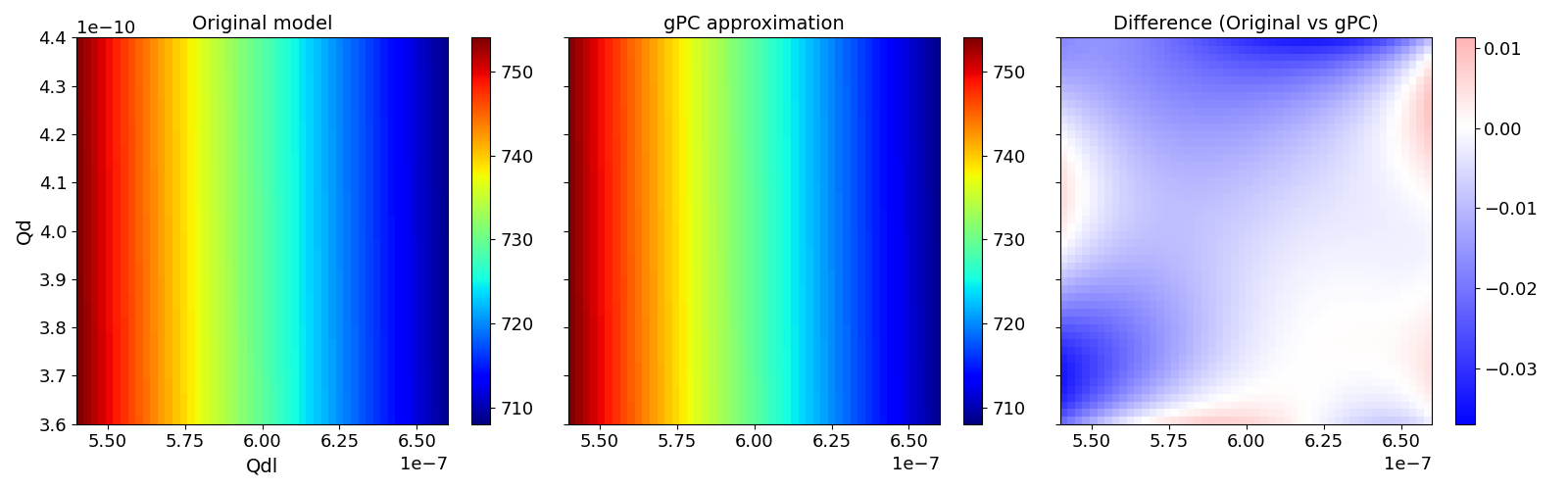
Validate gPC vs original model function (2D-surface)#
Validate gPC vs original model function
pygpc.validate_gpc_plot(session=session,
                        coeffs=coeffs,
                        random_vars=["Qdl", "Qd"],
                        n_grid=[51, 51],
                        output_idx=500,
                        fn_out=None,
                        n_cpu=session.n_cpu)
Validate gPC vs original model function (Monte Carlo)#
nrmsd = pygpc.validate_gpc_mc(session=session,
                              coeffs=coeffs,
                              n_samples=int(1e4),
                              output_idx=500,
                              n_cpu=session.n_cpu,
                              fn_out=fn_results)

print("> Maximum NRMSD (gpc vs original): {:.2}%".format(max(nrmsd)))
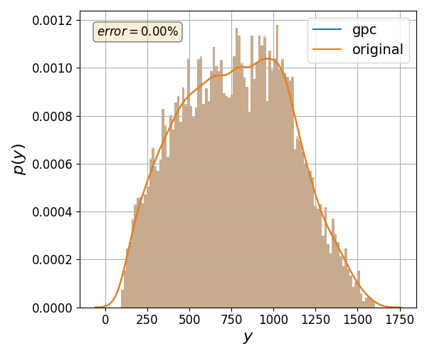
Out:
> Maximum NRMSD (gpc vs original): 2.6e-05%
Load sobol indices, mean and std from the *.hdf5 file#
import h5py

# Set parameters for plot
n_f = 1000
f_start = 0
f_stop = 9
f = np.logspace(f_start, f_stop, n_f)
legend = [r"$n_{Q_{dl}}$", r"$Q_{dl}$", r"$n_{Q_{d}}$", r"$Q_{d}$", r"$Rs$", r"$Rct$", r"$Rd$"]

# Set indices for quantities of interest
real_indices = np.arange(0, 1*n_f)
imag_indices = np.arange(1*n_f, 2*n_f)

# Load results file
file = h5py.File(fn_results + ".hdf5", "r")

# Load mean
mean = file["sens/mean"][()]

mean_real = np.squeeze(mean[:, real_indices].T)
mean_imag = np.squeeze(mean[:, imag_indices].T)

# Load std
std = file["sens/std"][()]

std_real = np.squeeze(std[:, real_indices].T)
std_imag = np.squeeze(std[:, imag_indices].T)

# Load boolean array that indicates which sensitivity coefficient corresponds to which parameter or
# interaction of parameters
sobol_index_bool = std = file["sens/sobol_idx_bool"][()]

# Get die sobol coefficients for interactions of first order i.e. just the parameter
n_Qdl_index_array = np.eye(7, 7)[0, :]
Qdl_index_array = np.eye(7, 7)[1, :]
n_Qd_index_array = np.eye(7, 7)[2, :]
Qd_index_array = np.eye(7, 7)[3, :]
Rs_index_array = np.eye(7, 7)[4, :]
Rct_index_array = np.eye(7, 7)[5, :]
Rd_index_array = np.eye(7, 7)[6, :]

n_Qdl_index = None
Qdl_index = None
n_Qd_index = None
Qd_index = None
Rs_index = None
Rct_index = None
Rd_index = None

for index in range(sobol_index_bool.shape[0]):
    if np.all(sobol_index_bool[index, :] == n_Qdl_index_array):
        n_Qdl_index = index
    if np.all(sobol_index_bool[index, :] == Qdl_index_array):
        Qdl_index = index
    if np.all(sobol_index_bool[index, :] == n_Qd_index_array):
        n_Qd_index = index
    if np.all(sobol_index_bool[index, :] == Qd_index_array):
        Qd_index = index
    if np.all(sobol_index_bool[index, :] == Rs_index_array):
        Rs_index = index
    if np.all(sobol_index_bool[index, :] == Rct_index_array):
        Rct_index = index
    if np.all(sobol_index_bool[index, :] == Rd_index_array):
        Rd_index = index


sobol_norm = std = file["sens/sobol_norm"][()]

sobol_norm_n_Qdl_real = sobol_norm[n_Qdl_index, real_indices]
sobol_norm_n_Qdl_imag = sobol_norm[n_Qdl_index, imag_indices]

sobol_norm_Qdl_real = sobol_norm[Qdl_index, real_indices]
sobol_norm_Qdl_imag = sobol_norm[Qdl_index, imag_indices]

sobol_norm_n_Qd_real = sobol_norm[n_Qd_index, real_indices]
sobol_norm_n_Qd_imag = sobol_norm[n_Qd_index, imag_indices]

sobol_norm_Qd_real = sobol_norm[Qd_index, real_indices]
sobol_norm_Qd_imag = sobol_norm[Qd_index, imag_indices]

sobol_norm_Rs_real = sobol_norm[Rs_index, real_indices]
sobol_norm_Rs_imag = sobol_norm[Rs_index, imag_indices]

sobol_norm_Rct_real = sobol_norm[Rct_index, real_indices]
sobol_norm_Rct_imag = sobol_norm[Rct_index, imag_indices]

sobol_norm_Rd_real = sobol_norm[Rd_index, real_indices]
sobol_norm_Rd_imag = sobol_norm[Rd_index, imag_indices]


# Print sum of first order sobol indices. The sum of all sobol indices must be equal to one
print("Minimum of sum of sobol indices of real part: ", np.min(sobol_norm_n_Qdl_real + sobol_norm_n_Qd_real +
      sobol_norm_Qd_real + sobol_norm_Qdl_real + sobol_norm_Rs_real + sobol_norm_Rct_real + sobol_norm_Rd_real))

print("Maximum of sum of sobol indices of real part: ", np.max(sobol_norm_n_Qdl_real + sobol_norm_n_Qd_real +
      sobol_norm_Qd_real + sobol_norm_Qdl_real + sobol_norm_Rs_real + sobol_norm_Rct_real + sobol_norm_Rd_real))

print("Mean of sum of sobol indices of real part: ", np.mean(sobol_norm_n_Qdl_real + sobol_norm_n_Qd_real +
      sobol_norm_Qd_real + sobol_norm_Qdl_real + sobol_norm_Rs_real + sobol_norm_Rct_real + sobol_norm_Rd_real))

print("Minimum of sum of sobol indices of imag part: ", np.min(sobol_norm_n_Qdl_imag + sobol_norm_n_Qd_imag +
      sobol_norm_Qd_imag + sobol_norm_Qdl_imag + sobol_norm_Rs_imag + sobol_norm_Rct_imag + sobol_norm_Rd_imag))

print("Maximum of sum of sobol indices of imag part: ", np.max(sobol_norm_n_Qdl_imag + sobol_norm_n_Qd_imag +
      sobol_norm_Qd_imag + sobol_norm_Qdl_imag + sobol_norm_Rs_imag + sobol_norm_Rct_imag + sobol_norm_Rd_imag))

print("Mean of sum of sobol indices of imag part: ", np.mean(sobol_norm_n_Qdl_imag + sobol_norm_n_Qd_imag +
      sobol_norm_Qd_imag + sobol_norm_Qdl_imag + sobol_norm_Rs_imag + sobol_norm_Rct_imag + sobol_norm_Rd_imag))

# Close file
file.close()
Out:
Minimum of sum of sobol indices of real part:  0.9922830860823648
Maximum of sum of sobol indices of real part:  0.9999999960849593
Mean of sum of sobol indices of real part:  0.9984816706723425
Minimum of sum of sobol indices of imag part:  0.95410545910002
Maximum of sum of sobol indices of imag part:  0.9988259205269608
Mean of sum of sobol indices of imag part:  0.995266507219882
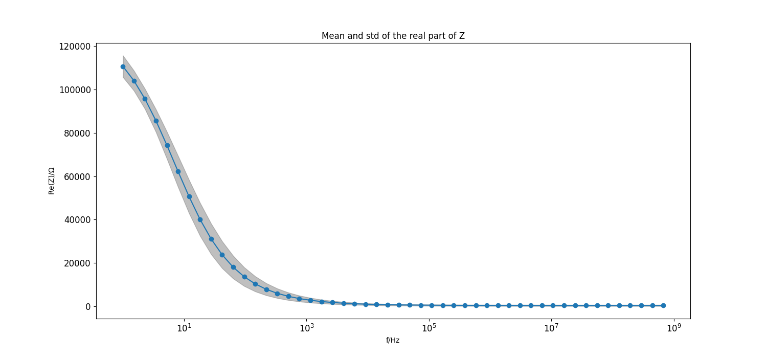
Plot mean and std of real part of the model#
Set step size for frequency points to plot
frequency_index_step = 20

# Plot mean and std of real part of the model
_ = plt.figure(figsize=[15, 7])
_ = plt.semilogx(f[::frequency_index_step], mean_real[::frequency_index_step], "C0o-")
_ = plt.fill_between(f[::frequency_index_step], mean_real[::frequency_index_step]-std_real[::frequency_index_step],
                     mean_real[::frequency_index_step]+std_real[::frequency_index_step],
                     color="grey", alpha=0.5)
_ = plt.title("Mean and std of the real part of Z")
_ = plt.xlabel("f/Hz")
_ = plt.ylabel(r"Re(Z)/$\Omega$")
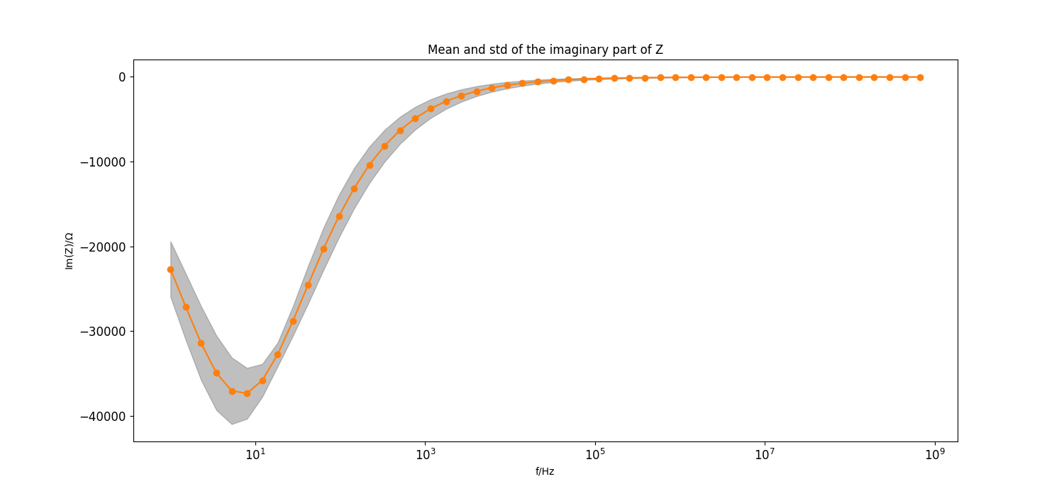
Plot mean and std of imaginary part of the model#
_ = plt.figure(figsize=[15, 7])
_ = plt.semilogx(f[::frequency_index_step], mean_imag[::frequency_index_step], "C1o-")
_ = plt.fill_between(f[::frequency_index_step], mean_imag[::frequency_index_step]-std_imag[::frequency_index_step], mean_imag[::frequency_index_step]+std_imag[::frequency_index_step],
                     color="grey", alpha=0.5)
_ = plt.title("Mean and std of the imaginary part of Z")
_ = plt.xlabel("f/Hz")
_ = plt.ylabel(r"Im(Z)/$\Omega$")
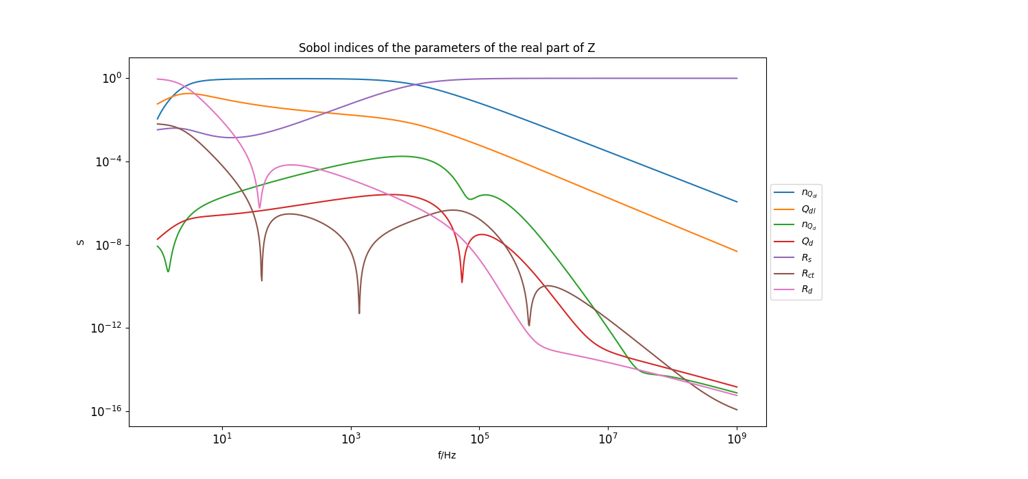
Plot sobol indices of the parameters of the real part of the model#
Set step size for frequency points to plot
frequency_index_step = 1

_ = plt.figure(figsize=[15, 7])

_ = plt.loglog(f[::frequency_index_step], sobol_norm_n_Qdl_real[::frequency_index_step], label=r"$n_{Q_{dl}}$")
_ = plt.loglog(f[::frequency_index_step], sobol_norm_Qdl_real[::frequency_index_step], label=r"$Q_{dl}$")
_ = plt.loglog(f[::frequency_index_step], sobol_norm_n_Qd_real[::frequency_index_step], label=r"$n_{Q_{d}}$")
_ = plt.loglog(f[::frequency_index_step], sobol_norm_Qd_real[::frequency_index_step], label=r"$Q_{d}}$")
_ = plt.loglog(f[::frequency_index_step], sobol_norm_Rs_real[::frequency_index_step], label=r"$R_s$")
_ = plt.loglog(f[::frequency_index_step], sobol_norm_Rct_real[::frequency_index_step], label=r"$R_{ct}$")
_ = plt.loglog(f[::frequency_index_step], sobol_norm_Rd_real[::frequency_index_step], label=r"$R_d$")
_ = plt.title("Sobol indices of the parameters of the real part of Z")
_ = plt.xlabel("f/Hz")
_ = plt.ylabel("S")

ax = plt.gca()
box = ax.get_position()
ax.set_position([box.x0, box.y0, box.width * 0.8, box.height])
ax.legend(loc='center left', bbox_to_anchor=(1, 0.5))
ylim_bottom, ylim_top = plt.ylim()
_ = plt.ylim([ylim_bottom, 10])
_ = plt.yticks(np.flip(np.logspace(int(np.floor(np.log10(ylim_bottom))), 0,
                                   int(np.abs(np.floor(np.log10(ylim_bottom))))+1))[::4])
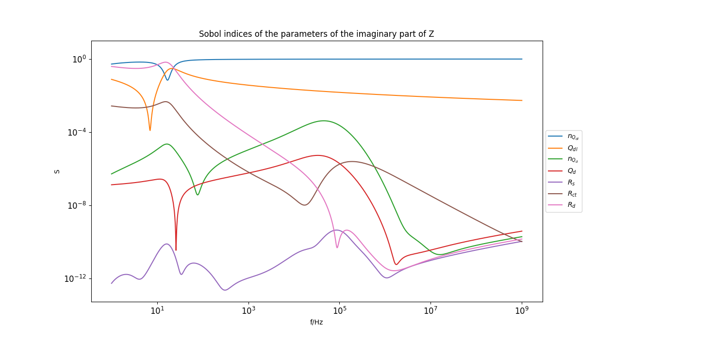
Plot sobol indices of the parameters of the imaginary part of the model#
_ = plt.figure(figsize=[15, 7])

_ = plt.loglog(f[::frequency_index_step], sobol_norm_n_Qdl_imag[::frequency_index_step], label=r"$n_{Q_{dl}}$")
_ = plt.loglog(f[::frequency_index_step], sobol_norm_Qdl_imag[::frequency_index_step], label=r"$Q_{dl}$")
_ = plt.loglog(f[::frequency_index_step], sobol_norm_n_Qd_imag[::frequency_index_step], label=r"$n_{Q_{d}}$")
_ = plt.loglog(f[::frequency_index_step], sobol_norm_Qd_imag[::frequency_index_step], label=r"$Q_{d}}$")
_ = plt.loglog(f[::frequency_index_step], sobol_norm_Rs_imag[::frequency_index_step], label=r"$R_s$")
_ = plt.loglog(f[::frequency_index_step], sobol_norm_Rct_imag[::frequency_index_step], label=r"$R_{ct}$")
_ = plt.loglog(f[::frequency_index_step], sobol_norm_Rd_imag[::frequency_index_step], label=r"$R_d$")
_ = plt.title("Sobol indices of the parameters of the imaginary part of Z")
_ = plt.xlabel("f/Hz")
_ = plt.ylabel("S")

ax = plt.gca()
box = ax.get_position()
ax.set_position([box.x0, box.y0, box.width * 0.8, box.height])
ax.legend(loc='center left', bbox_to_anchor=(1, 0.5))
ylim_bottom, ylim_top = plt.ylim()
_ = plt.ylim([ylim_bottom, 10])
_ = plt.yticks(np.flip(np.logspace(int(np.floor(np.log10(ylim_bottom))), 0,
                                   int(np.abs(np.floor(np.log10(ylim_bottom))))+1))[::4])

# On Windows subprocesses will import (i.e. execute) the main module at start.
# You need to insert an if __name__ == '__main__': guard in the main module to avoid
# creating subprocesses recursively.
#
# if __name__ == '__main__':
#     main()
Total running time of the script: ( 0 minutes 13.000 seconds)