Example: Lorenz system of differential equations (Julia)

About the model

This tutorial treats the same problem as in Example: Lorenz system of differential equations. In this tutorial, we show how to analyze julia functions with pygpc. The governing equations of the Lorenz system are:

\[ \begin{align}\begin{aligned}\frac{\partial x}{\partial t} &= \sigma (y - x)\\\frac{\partial y}{\partial t} &= x (\rho - z) - y\\\frac{\partial z}{\partial t} &= xy - \beta z\end{aligned}\end{align} \]

They are implemented in a julia .jl file that uses DifferentialEquations.jl as a dependency. The model .jl file contains the following:

using DifferentialEquations

function lorenz!(du,u,p,t)
    σ, β, ρ = p
    du[1] = σ*(u[2]-u[1])
    du[2] = u[1]*(ρ-u[3]) - u[2]
    du[3] = u[1]*u[2] - β*u[3]
   end

function Julia_Lorenz(p, u0, t_vals)
   tspan = (first(t_vals), last(t_vals))
   prob = ODEProblem(lorenz!,u0,tspan, p)
   sol = solve(prob)
   return sol(t_vals)
end

In order to analyze this model with pygpc, we have to set up a pygpc Model, which calls the aforementioned julia model file. In order to call the .jl file with pygpc, the Model has to be set up like in the following example. This code is implemented in Lorenz system (julia):

class Lorenz_System_julia(AbstractModel):

    # during initialization, the filename of the .jl model file is passed for further use
    def __init__(self, fname_julia=None):
        if fname_julia is not None:
            self.fname_julia = fname_julia
        self.fname = inspect.getfile(inspect.currentframe())

    def validate(self):
        pass

    def simulate(self, process_id=None, matlab_engine=None):

        from julia import Main

        # in this example, the package DifferentialEquations.jl needs to be installed in the
        # julia environment for this example the folder "julia_env" is located in the same
        # folder as the julia model file
        # if you installed the DifferentialEquations package by yourself in julia, you do not have to use a
        # dedicated environment (if julia updates, the environments also have to be updated from time to time
        # to keep working)

        #fname_folder = os.path.split(self.fname_julia)[0]
        #Main.fname_environment = os.path.join(fname_folder, 'julia_env')
        #Main.eval('import Pkg; Pkg.activate(fname_environment)')

        # access .jl file
        Main.fname_julia = self.fname_julia
        Main.include(Main.fname_julia)

        # create time and solution arrays
        n_grid = self.p["sigma"].shape[0]
        t = np.arange(0.0, self.p["t_end"][0], self.p["step_size"][0])
        sols = np.zeros((n_grid, t.shape[0]))

        # loop over parameter combinations and integrate differential equations
        for i in range(n_grid):
            # read parameters from self.p
            p = [self.p["sigma"][i], self.p["beta"][i], self.p["rho"][i]]

            # assign initial values (the same for all parameter combinations but pygpc duplicates
            # all "static" (deterministic) parameters for each parameter set)
            y0 = [self.p["x_0"][i], self.p["y_0"][i], self.p["z_0"][i]]

            # Call julia and save x-coordinate for this particular example (index 0)
            sols[i, :] = Main.Julia_Lorenz(p, y0, t)[0]

        x_out = sols

        return x_out

The model can then be called in the associated analysis script:

import os
import pygpc
import numpy as np
from collections import OrderedDict
import matplotlib
# matplotlib.use("Qt5Agg")

# Windows users have to encapsulate the code into a main function to avoid multiprocessing errors.
# def main():
fn_results = "tmp/example_lorenz_julia"

# define model
model = Lorenz_System_julia(fname_julia=os.path.join(pygpc.__path__[0], "testfunctions", "Lorenz_System.jl"))

# define problem
parameters = OrderedDict()
parameters["sigma"] = pygpc.Beta(pdf_shape=[1, 1], pdf_limits=[10-1, 10+1])
parameters["beta"] = pygpc.Beta(pdf_shape=[1, 1], pdf_limits=[28-10, 28+10])
parameters["rho"] = pygpc.Beta(pdf_shape=[1, 1], pdf_limits=[(8/3)-1, (8/3)+1])
parameters["x_0"] = 1.0
parameters["y_0"] = 1.0
parameters["z_0"] = 1.0
parameters["t_end"] = 5.0
parameters["step_size"] = 0.01

problem = pygpc.Problem(model, parameters)

# gPC options
options = dict()
options["order_start"] = 6
options["order_end"] = 20
options["solver"] = "Moore-Penrose"
options["interaction_order"] = 2
options["order_max_norm"] = 0.7
options["n_cpu"] = 0
options["error_type"] = 'nrmsd'
options["error_norm"] = 'absolute'
options["n_samples_validation"] = 1000
options["matrix_ratio"] = 5
options["fn_results"] = fn_results
options["eps"] = 0.01
options["grid_options"] = {"seed": 1}

# define algorithm
algorithm = pygpc.RegAdaptive(problem=problem, options=options)

# Initialize gPC Session
session = pygpc.Session(algorithm=algorithm)

# run gPC session
session, coeffs, results = session.run()

# Post-process gPC and add results to .hdf5 file
pygpc.get_sensitivities_hdf5(fn_gpc=session.fn_results,
                             output_idx=None,
                             calc_sobol=True,
                             calc_global_sens=True,
                             calc_pdf=False,
                             n_samples=int(1e4))

# get sobol indices
sobol, gsens = pygpc.get_sens_summary(fn_gpc=fn_results,
                                      parameters_random=session.parameters_random,
                                      fn_out=None)

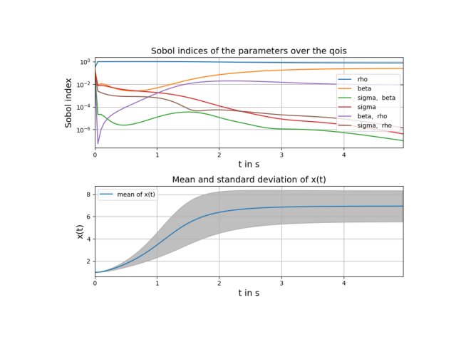
# plot sobol indices over time and mean and standard deviation of x(t)
t = np.arange(0.0, parameters["t_end"], parameters["step_size"])
pygpc.plot_sens_summary(session=session,
                        coeffs=coeffs,
                        sobol=sobol,
                        gsens=gsens,
                        plot_pdf_over_output_idx=True,
                        qois=t,
                        mean=pygpc.SGPC.get_mean(coeffs),
                        std=pygpc.SGPC.get_std(coeffs),
                        x_label="t in s",
                        y_label="x(t)",
                        zlim=[0, 0.4])

import matplotlib.pyplot as plt

# _ = plt.figure(figsize=[25, 10])
_ = plt.imshow(plt.imread("../images/Lorenz_Sobol.png"))
_ = plt.axis('off')



# On Windows subprocesses will import (i.e. execute) the main module at start.
# You need to insert an if __name__ == '__main__': guard in the main module to avoid
# creating subprocesses recursively.
#
# if __name__ == '__main__':
#     main()