Note
Go to the end to download the full example code.
Polynomial basis functions#
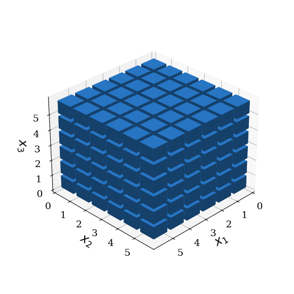
Total-order gPC#
In general, the set \(\mathcal{A}(\mathbf{p})\) of multi-indices can be freely chosen according to the problem under investigation. In the following figures, the blue boxes correspond to polynomials included in the gPC expansion. The coordinates of the boxes correspond to the multi-indices \(\mathbf{\alpha}\), which correspond to the polynomial degrees of the individual basis functions forming the joint basis functions. For a total-order gPC, the number of basis functions, and hence, coefficients to determine, increases exponentially in this case \(N_c=(p+1)^d\)
# Windows users have to encapsulate the code into a main function to avoid multiprocessing errors.
# def main():
import pygpc
import numpy as np
from IPython import display
from collections import OrderedDict

# define model
model = pygpc.testfunctions.Ishigami()

# define parameters
parameters = OrderedDict()
parameters["x1"] = pygpc.Beta(pdf_shape=[1, 1], pdf_limits=[-np.pi, np.pi])
parameters["x2"] = pygpc.Beta(pdf_shape=[1, 1], pdf_limits=[-np.pi, np.pi])
parameters["x3"] = pygpc.Beta(pdf_shape=[1, 1], pdf_limits=[-np.pi, np.pi])

# define problem
problem = pygpc.Problem(model, parameters)

# define basis
basis = pygpc.Basis()
basis.init_basis_sgpc(problem=problem,
                      order=[5, 5, 5],
                      order_max=15,
                      order_max_norm=1,
                      interaction_order=3)

basis.plot_basis(dims=[0, 1, 2])
/home/docs/checkouts/readthedocs.org/user_builds/pygpc/envs/latest/lib/python3.11/site-packages/pygpc/Basis.py:480: UserWarning: set_ticklabels() should only be used with a fixed number of ticks, i.e. after set_ticks() or using a FixedLocator.
  ax.set_xticklabels(range(np.max(multi_indices) + 1))
/home/docs/checkouts/readthedocs.org/user_builds/pygpc/envs/latest/lib/python3.11/site-packages/pygpc/Basis.py:482: UserWarning: set_ticklabels() should only be used with a fixed number of ticks, i.e. after set_ticks() or using a FixedLocator.
  ax.set_yticklabels(range(np.max(multi_indices) + 1))
/home/docs/checkouts/readthedocs.org/user_builds/pygpc/envs/latest/lib/python3.11/site-packages/pygpc/Basis.py:484: UserWarning: set_ticklabels() should only be used with a fixed number of ticks, i.e. after set_ticks() or using a FixedLocator.
  ax.set_zticklabels(range(np.max(multi_indices) + 1))
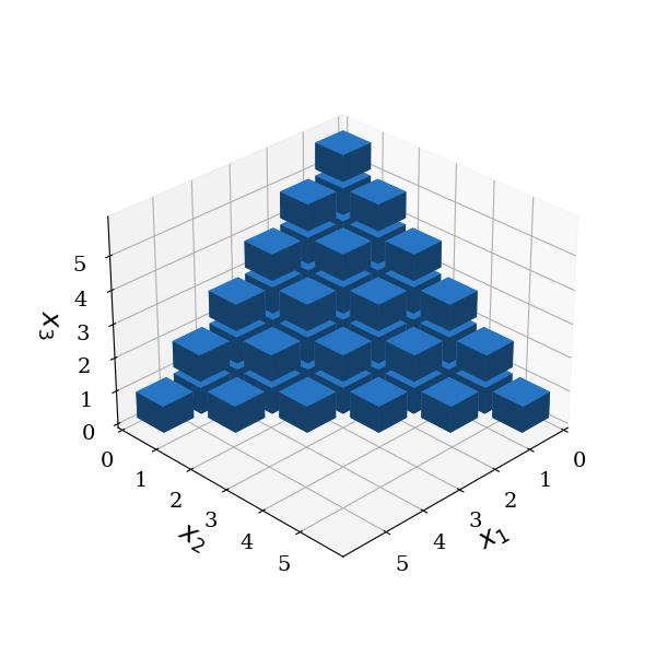
Maximum-order gPC#
In practical applications, the more economical maximum total order gPC is preferably used. In this case, the set \(\mathcal{A}(p_g)\) includes all polynomials whose total order does not exceed a predefined value \(p_g\).
This results in a reduced set of basis functions and is termed maximum order gPC. The number of multi-indices, and hence, the dimension of the space spanned by the polynomials, is:
basis = pygpc.Basis()
basis.init_basis_sgpc(problem=problem,
                      order=[5, 5, 5],
                      order_max=5,
                      order_max_norm=1,
                      interaction_order=3)

basis.plot_basis(dims=[0, 1, 2])
/home/docs/checkouts/readthedocs.org/user_builds/pygpc/envs/latest/lib/python3.11/site-packages/pygpc/Basis.py:480: UserWarning: set_ticklabels() should only be used with a fixed number of ticks, i.e. after set_ticks() or using a FixedLocator.
  ax.set_xticklabels(range(np.max(multi_indices) + 1))
/home/docs/checkouts/readthedocs.org/user_builds/pygpc/envs/latest/lib/python3.11/site-packages/pygpc/Basis.py:482: UserWarning: set_ticklabels() should only be used with a fixed number of ticks, i.e. after set_ticks() or using a FixedLocator.
  ax.set_yticklabels(range(np.max(multi_indices) + 1))
/home/docs/checkouts/readthedocs.org/user_builds/pygpc/envs/latest/lib/python3.11/site-packages/pygpc/Basis.py:484: UserWarning: set_ticklabels() should only be used with a fixed number of ticks, i.e. after set_ticks() or using a FixedLocator.
  ax.set_zticklabels(range(np.max(multi_indices) + 1))
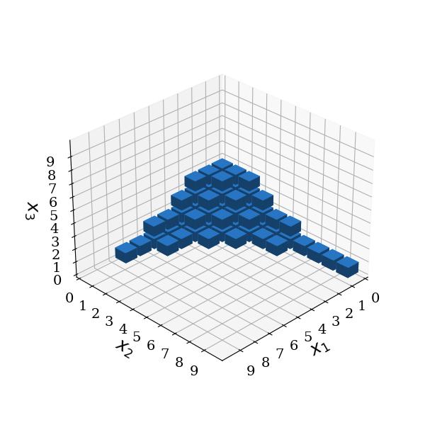
Reduced-basis gPC#
The concept of the maximum-order gPC is extended by introducing three new parameters: - the univariate expansion order \(\mathbf{p}_u = (p_{u,1},...,p_{u,d})\) with \(p_{u,i}>p_g \forall i={1,...,d}\) - the interaction order \(p_i\), limits the number of interacting parameters and it reflects the dimensionality, i.e. the number of random variables (independent variables) appearing in the basis function \(\Psi_{\mathbf{\alpha}}({\xi})\): \(\lVert\mathbf{\alpha}\rVert_0 \leq p_i\) - the maximum order norm \(q\) additionally truncates the included basis functions in terms of the maximum order \(p_g\) such that \(\lVert \mathbf{\alpha} \rVert_{q}=\sqrt[q]{\sum_{i=1}^d \alpha_i^{q}} \leq p_g\)
Those parameters define the set \(\mathcal{A}(\mathbf{p})\) with \(\mathbf{p} = (\mathbf{p}_u,p_i,p_g, q)\)
The reduced set \(\mathcal{A}(\mathbf{p})\) is then constructed by the following rule:
It includes all elements from a total order gPC with the restriction of the interaction order \(p_i\). Additionally, univariate polynomials of higher orders specified in \(\mathbf{p}_u\) may be added to the set of basis functions.
# reduced basis gPC
basis = pygpc.Basis()
basis.init_basis_sgpc(problem=problem,
                      order=[7, 9, 3],
                      order_max=7,
                      order_max_norm=0.8,
                      interaction_order=3)

basis.plot_basis(dims=[0, 1, 2])
/home/docs/checkouts/readthedocs.org/user_builds/pygpc/envs/latest/lib/python3.11/site-packages/pygpc/Basis.py:480: UserWarning: set_ticklabels() should only be used with a fixed number of ticks, i.e. after set_ticks() or using a FixedLocator.
  ax.set_xticklabels(range(np.max(multi_indices) + 1))
/home/docs/checkouts/readthedocs.org/user_builds/pygpc/envs/latest/lib/python3.11/site-packages/pygpc/Basis.py:482: UserWarning: set_ticklabels() should only be used with a fixed number of ticks, i.e. after set_ticks() or using a FixedLocator.
  ax.set_yticklabels(range(np.max(multi_indices) + 1))
/home/docs/checkouts/readthedocs.org/user_builds/pygpc/envs/latest/lib/python3.11/site-packages/pygpc/Basis.py:484: UserWarning: set_ticklabels() should only be used with a fixed number of ticks, i.e. after set_ticks() or using a FixedLocator.
  ax.set_zticklabels(range(np.max(multi_indices) + 1))
Isotropic adaptive basis#
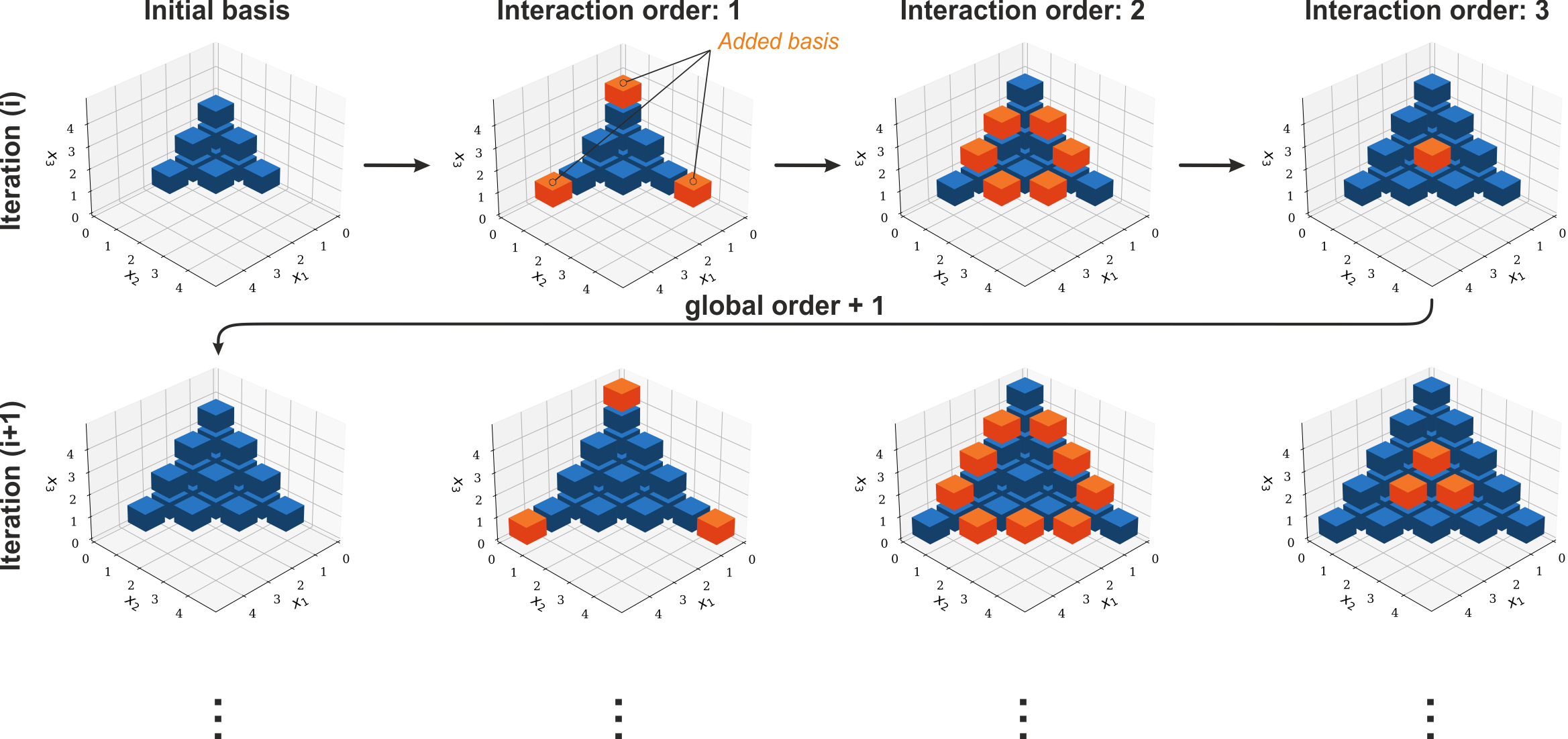
The basic problem in gPC is to find a suitable basis while reducing the number of necessary forward simulations to determine the gPC coefficients! To do this two basis increment strategies exist. This first is called isotropic and is the default option for the gpc. It determines which multi-indices are picked to be added to the existing set of basis functions in terms of their order and dimension. The boundary conditions for this expansion are given by the maximum order and the interaction order in the gpc options. The maximum order sets a limit to how high any index may grow and the interaction order limits the maximal dimension in which multi-indices can be chosen. In action isotropic basis incrementation chooses the new basis multi-indices equally in each direction decreasing the dimension in every step. If the interaction order is set as 3 this means that the first indices to be increased is along the axes (shown in orange in the figure below), then the indices that span the area between the axes are chosen and finally the indices that create the volume contained by the surrounding area are added. After that the axes are extended again and the cycle is repeated until the error is sufficient. For an interaction order of higher than three the expansion continues until the final dimension is reached.
# define model
model = pygpc.testfunctions.Ishigami()

# define problem
parameters = OrderedDict()
parameters["x1"] = pygpc.Beta(pdf_shape=[1, 1], pdf_limits=[-np.pi, np.pi])
parameters["x2"] = pygpc.Beta(pdf_shape=[1, 1], pdf_limits=[-np.pi, np.pi])
parameters["x3"] = pygpc.Beta(pdf_shape=[1, 1], pdf_limits=[-np.pi, np.pi])
parameters["a"] = 7.
parameters["b"] = 0.1

problem = pygpc.Problem(model, parameters)

# gPC options
options = dict()
options["order_start"] = 10
options["order_end"] = 20
options["solver"] = "Moore-Penrose"
options["interaction_order"] = 2
options["order_max_norm"] = 1.0
options["n_cpu"] = 0
options["adaptive_sampling"] = False
options["eps"] = 0.05
options["fn_results"] = None
options["basis_increment_strategy"] = None
options["matrix_ratio"] = 4
options["grid"] = pygpc.Random
options["grid_options"] = {"seed": 1}

# define algorithm
algorithm = pygpc.RegAdaptive(problem=problem, options=options)

# Initialize gPC Session
session = pygpc.Session(algorithm=algorithm)

# run gPC session
session, coeffs, results = session.run()
Initializing gPC object...
Creating initial grid (Random) with n_grid=664
Initializing gPC matrix...
Extending grid from 664 to 664 by 0 sampling points
Performing simulations 1 to 664

It/Sub-it: 10/2 Performing simulation 001 from 664 [                                        ] 0.2%
Total parallel function evaluation: 0.00024962425231933594 sec
Determine gPC coefficients using 'Moore-Penrose' solver ...
-> relative loocv error = 0.004596157433886055
Determine gPC coefficients using 'Moore-Penrose' solver ...
Anisotropic adaptive basis#
In addition to the adaptive selection from the previous method, the specification options[“basis_increment_strategy”] = anisotropic can be used for the gpc object to use an algorithm by Gerstner and Griebel [1] for an anisotropic basis increment strategy. The motivation behind it lies in reducing the variance of the output data of the gpc.
where \(\mathbf{q}(\mathbf{\xi})\) is the output data dependent on \(\mathbf{\xi}\) which are the random variables, \(P\) is the order of the gpc and \(\mathbf{u}_{\mathbf{\alpha}_k}\) are the coefficients of the basis function \(\mathbf{\Phi}_{\mathbf{\alpha}_k}\). The variance depends directly on the coefficients \(\mathbf{u}_{\mathbf{\alpha}_k}\) and can be reduced by using them as a optimization criterion in the mentioned algorithm. A normalized version \(\hat{\mathbf{u}}_{\mathbf{\alpha}_k}\) directly corresponds to the variance and is given by
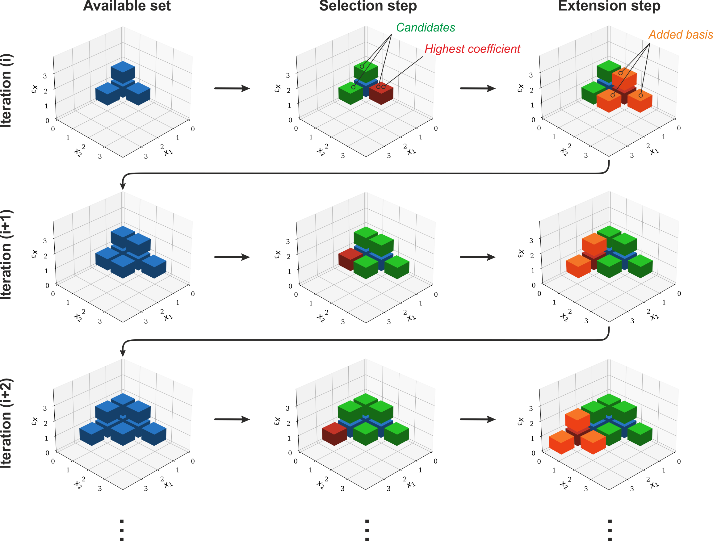
In pygpc this quantity is calculated as the maximum L2-norm of the current coefficients and the relevant index :math:’k’ is extracted from the set of multi-indices. The anisotropic adaptive basis algorithm selects the multi-index :math:’k’ with the highest norm as the starting point for a basis expansion. The goal during the expansion is to find suitable candidate indices that meet the following two criteria: (1) The index is not completely enclosed by other indices with higher basis components since this would mean that it is already included; (2) The index needs to have predecessors. This means that in all directions of decreasing order connecting multi-indices exist already and the new index is not ‘floating’. In the figure below this is shown again for the three-dimensional case. First the outer multi-indices that have connected faces with other included multi-indices which ‘have predecessors’ are selected (marked green). Then the basis function coefficients are computed for these candidates and the multi-index with the highest coefficient is picked for the expansion (marked red). The index is then expanded in every dimension around it where the resulting index is not already included in the multi-index-set yet (marked orange).
# define model
model = pygpc.testfunctions.Ishigami()

# define problem
parameters = OrderedDict()
parameters["x1"] = pygpc.Beta(pdf_shape=[1, 1], pdf_limits=[-np.pi, np.pi])
parameters["x2"] = pygpc.Beta(pdf_shape=[1, 1], pdf_limits=[-np.pi, np.pi])
parameters["x3"] = pygpc.Beta(pdf_shape=[1, 1], pdf_limits=[-np.pi, np.pi])
parameters["a"] = 7.
parameters["b"] = 0.1

problem = pygpc.Problem(model, parameters)

# gPC options
options = dict()
options["order_start"] = 10
options["order_end"] = 20
options["solver"] = "Moore-Penrose"
options["interaction_order"] = 2
options["order_max_norm"] = 1.0
options["n_cpu"] = 0
options["adaptive_sampling"] = False
options["eps"] = 0.05
options["fn_results"] = None
options["basis_increment_strategy"] = "anisotropic"
options["matrix_ratio"] = 4
options["grid"] = pygpc.Random
options["grid_options"] = {"seed": 1}

# define algorithm
algorithm = pygpc.RegAdaptive(problem=problem, options=options)

# Initialize gPC Session
session = pygpc.Session(algorithm=algorithm)

# run gPC session
session, coeffs, results = session.run()

#
#
# On Windows subprocesses will import (i.e. execute) the main module at start.
# You need to insert an if __name__ == '__main__': guard in the main module to avoid
# creating subprocesses recursively.
#
# if __name__ == '__main__':
#     main()
Initializing gPC object...
Creating initial grid (Random) with n_grid=664
Initializing gPC matrix...
Extending grid from 664 to 664 by 0 sampling points
Performing simulations 1 to 664

It/Sub-it: 10/2 Performing simulation 001 from 664 [                                        ] 0.2%
Total parallel function evaluation: 0.00025725364685058594 sec
Determine gPC coefficients using 'Moore-Penrose' solver ...
-> relative loocv error = 0.005596322463061914
Determine gPC coefficients using 'Moore-Penrose' solver ...
Total running time of the script: (0 minutes 2.405 seconds)