Note
Go to the end to download the full example code.
Modelling discontinuous model functions#
In some cases, the output quantities of a model are discontinuous in the investigated parameter ranges. Modelling such systems with global continuous basis polynomials of a classical gPC would require a very high polynomial order and consequently a large number of sampling points. In addition, discontinuities can only be modeled to a limited extent due to the Gibbs phenomenon (overshooting). The gPC approach has been extended by a multi-element approach (ME-gPC) so that this class of problems can also be analyzed efficiently using gPC. The approach consists of dividing the global parameter space into several regions in which the model function is continuous. Each of these regions is described with an independent gPC approach as it shown in the following example.
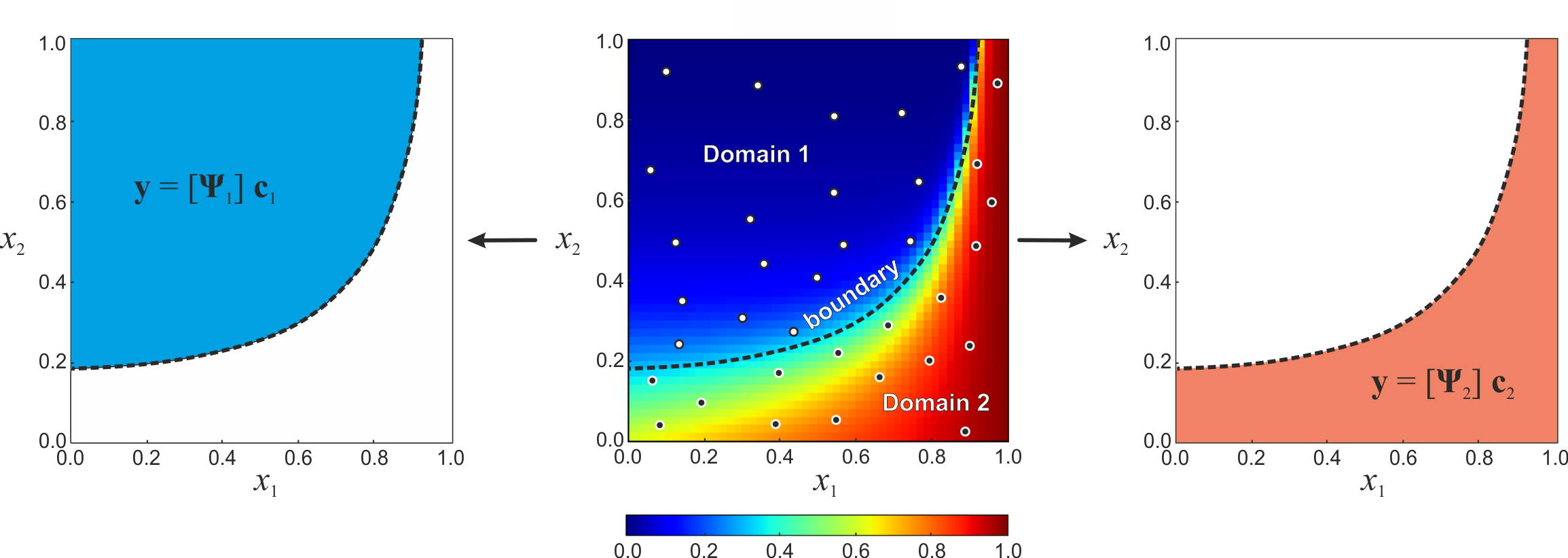
The core task of the method is to identify the discontinuity boundary between the regions. For this purpose, modern image processing and machine learning techniques are used. In a first step, a cluster analysis is performed based on the feature values at the sampling points and a class is assigned to each sample (unsupervised learning) depending on its function value. In a second step, the identified groups are used with a classification algorithm to identify the discontinuity boundary (supervised learning). This allowed, for example, uncertainty and sensitivity analysis of Jansen-Rit type neural mass models and created the basis for the analysis of this class of problems (Weise et al. 2020).
The post-processing and sensitivity analysis methods recognize if a multi-element gPC approach is used and adapts the calculation of the sensitivity coefficients according to the different domains using a sampling based approach instead of determining the sensitivity coefficients directly from the gPC coefficients.
In the following, an example of a discontinuous test problem is provided:
# Windows users have to encapsulate the code into a main function to avoid multiprocessing errors.
# def main():
import pygpc
from collections import OrderedDict
import matplotlib
# matplotlib.use("Qt5Agg")

fn_results = 'tmp/mestatic'       # filename of output
save_session_format = ".pkl"      # file format of saved gpc session ".hdf5" (slow) or ".pkl" (fast)
Loading the model and defining the problem#
# define model
model = pygpc.testfunctions.SurfaceCoverageSpecies()

# define problem
parameters = OrderedDict()
parameters["rho_0"] = pygpc.Beta(pdf_shape=[1, 1], pdf_limits=[0, 1])
parameters["beta"] = pygpc.Beta(pdf_shape=[1, 1], pdf_limits=[0, 20])
parameters["alpha"] = 1.
problem = pygpc.Problem(model, parameters)
Setting up the algorithm#
# gPC options
options = dict()
options["method"] = "reg"
options["solver"] = "Moore-Penrose"
options["settings"] = None
options["order"] = [10, 10]
options["order_max"] = 10
options["interaction_order"] = 2
options["n_cpu"] = 0
options["gradient_enhanced"] = False
options["error_type"] = "loocv"

# all QoIs are treated separately (one ME-gPC for each QoI, in this example we only have one QoI)
options["qoi"] = "all"

# Multi-Element classifier type is "learning"
options["classifier"] = "learning"

# set the options of the clusterer and classifier
options["classifier_options"] = {"clusterer": "KMeans",
                                 "n_clusters": 2,
                                 "classifier": "MLPClassifier",
                                 "classifier_solver": "lbfgs"}
“clusterer”: For clustering (unsupervised learning) we choose “KMeans” from sklearn.cluster.KMeans The clusterer assigns a domain ID to each sampling point depending on the function value.
“n_clusters”: number of different domains
“classifier”: For classification (supervised learning) we choose “MLPClassifier” from sklearn.neural_network.MLPClassifier With the domain IDs from the clusterer and the associated parameter values of the sampling points, a classifier is created, which can assign a domain ID to unknown (new) grid points.
“classifier_solver”: The solver of the classifier for weight optimization. (“lbfgs” is an optimizer in the family of quasi-Newton methods; “sgd” refers to stochastic gradient descent; “adam” refers to a stochastic gradient-based optimizer from Kingma and Ba (2014))
options["fn_results"] = fn_results
options["save_session_format"] = save_session_format
options["grid"] = pygpc.Random
options["grid_options"] = {"seed": 1}
options["n_grid"] = 1000
options["adaptive_sampling"] = False
We are going to use a static gPC approach here without any basis adaption. Algorithms, which include the multi-element gPC approach are:
Algorithm: MEStatic (standard gPC approach with static basis)
Algorithm: MEStatic_IO (standard gPC approach with static basis but precalculated input/output relationships)
Algorithm: MEStaticProjection (standard gPC approach with dimensionality reduction approach in each domain)
Algorithm: MERegAdaptiveProjection (adaptive basis approach with dimensionality reduction approach in each domain)
# define algorithm
algorithm = pygpc.MEStatic(problem=problem, options=options)
Running the gpc#
# Initialize gPC Session
session = pygpc.Session(algorithm=algorithm)

# run gPC algorithm
session, coeffs, results = session.run()
Creating initial grid (Random) with n_grid=1000
Determining gPC approximation for QOI #0:
=========================================
Performing 1000 simulations!

It/Sub-it: 10/2 Performing simulation 0001 from 1000 [                                        ] 0.1%
Total function evaluation: 0.4336864948272705 sec
Determine gPC coefficients using 'Moore-Penrose' solver ...
Determine gPC coefficients using 'Moore-Penrose' solver ...

LOOCV 01 from 25 [=                                       ] 4.0%

LOOCV 02 from 25 [===                                     ] 8.0%

LOOCV 03 from 25 [====                                    ] 12.0%

LOOCV 04 from 25 [======                                  ] 16.0%

LOOCV 05 from 25 [========                                ] 20.0%

LOOCV 06 from 25 [=========                               ] 24.0%

LOOCV 07 from 25 [===========                             ] 28.0%

LOOCV 08 from 25 [============                            ] 32.0%

LOOCV 09 from 25 [==============                          ] 36.0%

LOOCV 10 from 25 [================                        ] 40.0%

LOOCV 11 from 25 [=================                       ] 44.0%

LOOCV 12 from 25 [===================                     ] 48.0%

LOOCV 13 from 25 [====================                    ] 52.0%

LOOCV 14 from 25 [======================                  ] 56.0%

LOOCV 15 from 25 [========================                ] 60.0%

LOOCV 16 from 25 [=========================               ] 64.0%

LOOCV 17 from 25 [===========================             ] 68.0%

LOOCV 18 from 25 [============================            ] 72.0%

LOOCV 19 from 25 [==============================          ] 76.0%

LOOCV 20 from 25 [================================        ] 80.0%

LOOCV 21 from 25 [=================================       ] 84.0%

LOOCV 22 from 25 [===================================     ] 88.0%

LOOCV 23 from 25 [====================================    ] 92.0%

LOOCV 24 from 25 [======================================  ] 96.0%

LOOCV 25 from 25 [========================================] 100.0%
LOOCV computation time: 0.06536412239074707 sec
-> relative loocv error = 0.0558652368427167

LOOCV 01 from 25 [=                                       ] 4.0%

LOOCV 02 from 25 [===                                     ] 8.0%

LOOCV 03 from 25 [====                                    ] 12.0%

LOOCV 04 from 25 [======                                  ] 16.0%

LOOCV 05 from 25 [========                                ] 20.0%

LOOCV 06 from 25 [=========                               ] 24.0%

LOOCV 07 from 25 [===========                             ] 28.0%

LOOCV 08 from 25 [============                            ] 32.0%

LOOCV 09 from 25 [==============                          ] 36.0%

LOOCV 10 from 25 [================                        ] 40.0%

LOOCV 11 from 25 [=================                       ] 44.0%

LOOCV 12 from 25 [===================                     ] 48.0%

LOOCV 13 from 25 [====================                    ] 52.0%

LOOCV 14 from 25 [======================                  ] 56.0%

LOOCV 15 from 25 [========================                ] 60.0%

LOOCV 16 from 25 [=========================               ] 64.0%

LOOCV 17 from 25 [===========================             ] 68.0%

LOOCV 18 from 25 [============================            ] 72.0%

LOOCV 19 from 25 [==============================          ] 76.0%

LOOCV 20 from 25 [================================        ] 80.0%

LOOCV 21 from 25 [=================================       ] 84.0%

LOOCV 22 from 25 [===================================     ] 88.0%

LOOCV 23 from 25 [====================================    ] 92.0%

LOOCV 24 from 25 [======================================  ] 96.0%

LOOCV 25 from 25 [========================================] 100.0%
LOOCV computation time: 0.06804442405700684 sec

LOOCV 01 from 25 [=                                       ] 4.0%

LOOCV 02 from 25 [===                                     ] 8.0%

LOOCV 03 from 25 [====                                    ] 12.0%

LOOCV 04 from 25 [======                                  ] 16.0%

LOOCV 05 from 25 [========                                ] 20.0%

LOOCV 06 from 25 [=========                               ] 24.0%

LOOCV 07 from 25 [===========                             ] 28.0%

LOOCV 08 from 25 [============                            ] 32.0%

LOOCV 09 from 25 [==============                          ] 36.0%

LOOCV 10 from 25 [================                        ] 40.0%

LOOCV 11 from 25 [=================                       ] 44.0%

LOOCV 12 from 25 [===================                     ] 48.0%

LOOCV 13 from 25 [====================                    ] 52.0%

LOOCV 14 from 25 [======================                  ] 56.0%

LOOCV 15 from 25 [========================                ] 60.0%

LOOCV 16 from 25 [=========================               ] 64.0%

LOOCV 17 from 25 [===========================             ] 68.0%

LOOCV 18 from 25 [============================            ] 72.0%

LOOCV 19 from 25 [==============================          ] 76.0%

LOOCV 20 from 25 [================================        ] 80.0%

LOOCV 21 from 25 [=================================       ] 84.0%

LOOCV 22 from 25 [===================================     ] 88.0%

LOOCV 23 from 25 [====================================    ] 92.0%

LOOCV 24 from 25 [======================================  ] 96.0%

LOOCV 25 from 25 [========================================] 100.0%
LOOCV computation time: 0.04147171974182129 sec
Postprocessing#
# read session
session = pygpc.read_session(fname=session.fn_session, folder=session.fn_session_folder)

# Post-process gPC
pygpc.get_sensitivities_hdf5(fn_gpc=options["fn_results"],
                             output_idx=None,
                             calc_sobol=True,
                             calc_global_sens=True,
                             calc_pdf=True,
                             algorithm="sampling",
                             n_samples=1e4)
> Loading gpc session object: tmp/mestatic.pkl
> Loading gpc coeffs: tmp/mestatic.hdf5
> Adding results to: tmp/mestatic.hdf5
Validation#
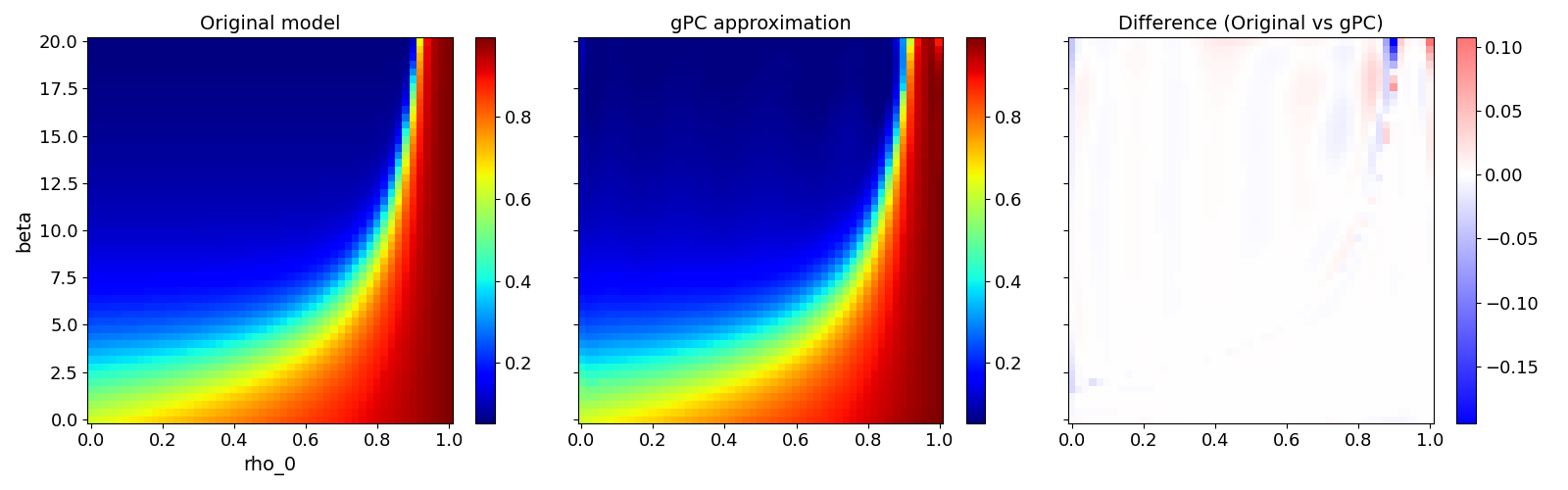
Validate gPC vs original model function (2D-surface)#
pygpc.validate_gpc_plot(session=session,
                        coeffs=coeffs,
                        random_vars=list(problem.parameters_random.keys()),
                        n_grid=[51, 51],
                        output_idx=[0],
                        fn_out=None,
                        folder=None,
                        n_cpu=session.n_cpu)
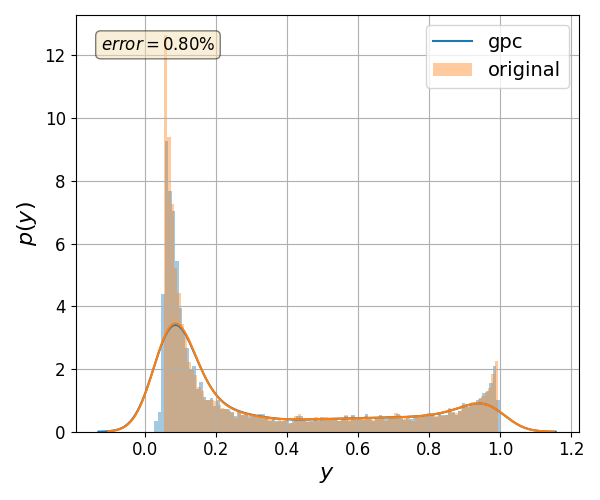
Validate gPC vs original model function (Monte Carlo)#
nrmsd = pygpc.validate_gpc_mc(session=session,
                              coeffs=coeffs,
                              n_samples=int(1e4),
                              output_idx=[0],
                              fn_out=None,
                              folder=None,
                              plot=True,
                              n_cpu=session.n_cpu)

print("> Maximum NRMSD (gpc vs original): {:.2}%".format(max(nrmsd)))
/home/docs/checkouts/readthedocs.org/user_builds/pygpc/envs/latest/lib/python3.11/site-packages/pygpc/validation.py:172: UserWarning:

`distplot` is a deprecated function and will be removed in seaborn v0.14.0.

Please adapt your code to use either `displot` (a figure-level function with
similar flexibility) or `histplot` (an axes-level function for histograms).

For a guide to updating your code to use the new functions, please see
https://gist.github.com/mwaskom/de44147ed2974457ad6372750bbe5751

  sns.distplot(y_gpc[:, i].flatten(), bins=bins, ax=ax1)
/home/docs/checkouts/readthedocs.org/user_builds/pygpc/envs/latest/lib/python3.11/site-packages/pygpc/validation.py:173: UserWarning:

`distplot` is a deprecated function and will be removed in seaborn v0.14.0.

Please adapt your code to use either `displot` (a figure-level function with
similar flexibility) or `histplot` (an axes-level function for histograms).

For a guide to updating your code to use the new functions, please see
https://gist.github.com/mwaskom/de44147ed2974457ad6372750bbe5751

  sns.distplot(y_orig[:, i].flatten(), bins=bins, label=r'original', ax=ax1)
> Maximum NRMSD (gpc vs original): 0.0068%
Sensitivity analysis#
sobol, gsens = pygpc.get_sens_summary(fn_results, problem.parameters_random)
pygpc.plot_sens_summary(sobol=sobol, gsens=gsens)
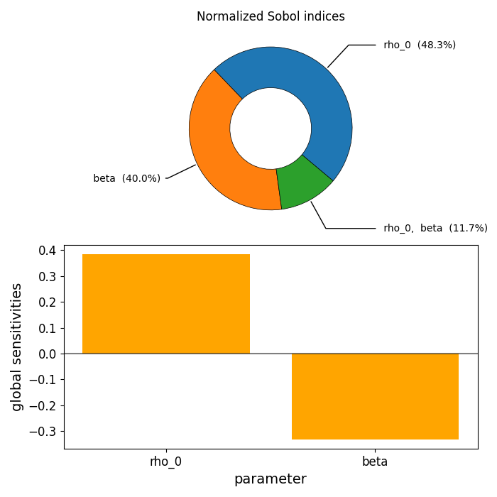
The Sobol indices at the top indicate that both parameters are influencing the output quantity by more than 40%. The global (derivative based) sensitivity coefficients at the bottom reveal that an increase in parameter rho_0 increases the model function and an increase of beta decreases the model function to almost the same extent. This can also be observed when taking a closer look at the model function in one of the previous figures.
# On Windows subprocesses will import (i.e. execute) the main module at start.
# You need to insert an if __name__ == '__main__': guard in the main module to avoid
# creating subprocesses recursively.
#
# if __name__ == '__main__':
#     main()
References#
Total running time of the script: (0 minutes 8.287 seconds)