Example: Ishigami Testfunction

About the model

This easy tutorial shows the application of pygpc to the Ishigami function, which can be found in the testfunctions section. The model consists of three random variables that are considered as input parameters (x1, x2, x3). The shape parameters of the function are chosen to be a=7 and b=0.1.

The model returns an output array with a value y for every sampling point.

# Windows users have to encapsulate the code into a main function to avoid multiprocessing errors.
# def main():

import os
import pygpc
import numpy as np
from collections import OrderedDict
import matplotlib
# matplotlib.use("Qt5Agg")

fn_results = "tmp/example_ishigami"

if os.path.exists(fn_results + ".hdf5"):
    os.remove(fn_results + ".hdf5")

if os.path.exists(fn_results + "_val.hdf5"):
    os.remove(fn_results + "_val.hdf5")

if os.path.exists(fn_results + "_mc.hdf5"):
    os.remove(fn_results + "_mc.hdf5")

# define model
model = pygpc.testfunctions.Ishigami()

# define problem
parameters = OrderedDict()
parameters["x1"] = pygpc.Beta(pdf_shape=[1, 1], pdf_limits=[-np.pi, np.pi])
parameters["x2"] = pygpc.Beta(pdf_shape=[1, 1], pdf_limits=[-np.pi, np.pi])
parameters["x3"] = pygpc.Beta(pdf_shape=[1, 1], pdf_limits=[-np.pi, np.pi])
parameters["a"] = 7.
parameters["b"] = 0.1

parameters_random = OrderedDict()
parameters_random["x1"] = pygpc.Beta(pdf_shape=[1, 1], pdf_limits=[-np.pi, np.pi])
parameters_random["x2"] = pygpc.Beta(pdf_shape=[1, 1], pdf_limits=[-np.pi, np.pi])
parameters_random["x3"] = pygpc.Beta(pdf_shape=[1, 1], pdf_limits=[-np.pi, np.pi])

problem = pygpc.Problem(model, parameters)

# gPC options
options = dict()
options["order"] = [15] * problem.dim
options["order_max"] = 15
options["order_start"] = 15
options["method"] = 'reg'
options["solver"] = "Moore-Penrose"
options["interaction_order"] = 2
options["order_max_norm"] = 1.0
options["n_cpu"] = 0
options["eps"] = 0.01
options["fn_results"] = fn_results
options["basis_increment_strategy"] = None
options["plot_basis"] = False
options["n_grid"] = 1300
options["save_session_format"] = ".pkl"
options["matrix_ratio"] = 2
options["grid"] = pygpc.Random
options["grid_options"] = {"seed": 1}

# define algorithm
algorithm = pygpc.Static(problem=problem, options=options, grid=None)

# Initialize gPC Session
session = pygpc.Session(algorithm=algorithm)

# run gPC session
session, coeffs, results = session.run()

Performing 1300 simulations!

It/Sub-it: 15/2 Performing simulation 0001 from 1300 [                                        ] 0.1%
Total parallel function evaluation: 0.0004019737243652344 sec
Determine gPC coefficients using 'Moore-Penrose' solver ...
-> relative loocv error = 1.6353509020631042e-05

Postprocessing

Postprocess gPC and add results to .hdf5 file

pygpc.get_sensitivities_hdf5(fn_gpc=session.fn_results,
                             output_idx=None,
                             calc_sobol=True,
                             calc_global_sens=True,
                             calc_pdf=True,
                             n_samples=int(1e4))

> Loading gpc session object: tmp/example_ishigami.pkl
> Loading gpc coeffs: tmp/example_ishigami.hdf5
> Adding results to: tmp/example_ishigami.hdf5

Validation

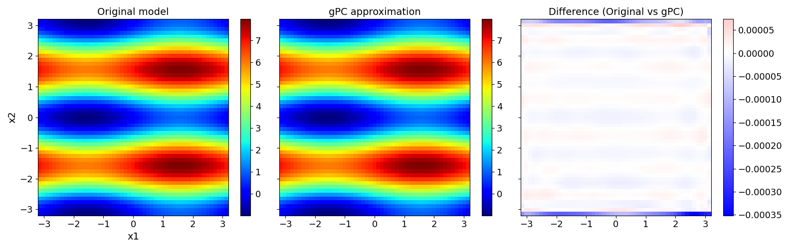
Validate gPC vs original model function

pygpc.validate_gpc_plot(session=session,
                        coeffs=coeffs,
                        random_vars=["x1", "x2"],
                        n_grid=[51, 51],
                        output_idx=0,
                        fn_out=session.fn_results + '_val',
                        n_cpu=session.n_cpu)

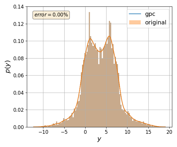
Validate gPC vs original model function (Monte Carlo)

nrmsd = pygpc.validate_gpc_mc(session=session,
                              coeffs=coeffs,
                              n_samples=int(1e4),
                              output_idx=0,
                              n_cpu=session.n_cpu,
                              fn_out=session.fn_results + '_mc')

/home/docs/checkouts/readthedocs.org/user_builds/pygpc/envs/latest/lib/python3.11/site-packages/pygpc/validation.py:172: UserWarning:

`distplot` is a deprecated function and will be removed in seaborn v0.14.0.

Please adapt your code to use either `displot` (a figure-level function with
similar flexibility) or `histplot` (an axes-level function for histograms).

For a guide to updating your code to use the new functions, please see
https://gist.github.com/mwaskom/de44147ed2974457ad6372750bbe5751

  sns.distplot(y_gpc[:, i].flatten(), bins=bins, ax=ax1)
/home/docs/checkouts/readthedocs.org/user_builds/pygpc/envs/latest/lib/python3.11/site-packages/pygpc/validation.py:173: UserWarning:

`distplot` is a deprecated function and will be removed in seaborn v0.14.0.

Please adapt your code to use either `displot` (a figure-level function with
similar flexibility) or `histplot` (an axes-level function for histograms).

For a guide to updating your code to use the new functions, please see
https://gist.github.com/mwaskom/de44147ed2974457ad6372750bbe5751

  sns.distplot(y_orig[:, i].flatten(), bins=bins, label=r'original', ax=ax1)

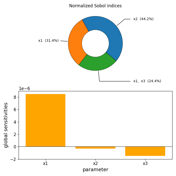
Sensitivity analysis

sobol, gsens = pygpc.get_sens_summary(fn_results, parameters_random, fn_results + "_sens_summary.txt")
pygpc.plot_sens_summary(sobol=sobol, gsens=gsens)

#
# On Windows subprocesses will import (i.e. execute) the main module at start.
# You need to insert an if __name__ == '__main__': guard in the main module to avoid
# creating subprocesses recursively.
#
# if __name__ == '__main__':
#     main()