Latin Hypercube Sampling (LHS)

To prevent clustering or undersampling of specific regions in the probability space, LHS is a simple alternative to enhance the space-filling properties of the sampling scheme first established by McKay et al. (2000).

To draw \(n\) independent samples from a number of \(d\)-dimensional parameters a matrix \(\Pi\) is constructed with

\[\pi_{ij} = \frac{p_{ij} - u}{n}\]

where \(P\) is a \(d \times n\) matrix of randomly perturbed integers \(p_{ij} \in \mathbb{N}, {1,...,n}\) and u is uniform random number \(u \in [0,1]\).

LHS Designs can further be improved upon, since the pseudo-random sampling procedure can lead to samples with high spurious correlation and the space filling capability in itself leaves room for improvement, some optimization criteria have been found to be adequate for compensating the initial designs shortcomings.

Optimization Criteria of LHS designs

Spearman Rank Correlation

For a sample size of \(n\) the scores of each variable are converted to their Ranks \(rg_{X_i}\) the Spearman Rank Correlation Coefficient is then the Pearson Correlation Coefficient applied to the rank variables \(rg_{X_i}\):

\[r_s = \rho_{rg_{X_i}, rg_{X_j}} = \frac{cov(rg_{X_i}, rg_{X_j})}{\sigma_{rg_{X_i}} \sigma_{rg_{X_i}}}\]

where \(\rho\) is the pearson correlation coefficient, \(\sigma\) is the standard deviation and \(cov\) is the covariance of the rank variables.

Maximum-Minimal-Distance

For creating a so called maximin distance design that maximizes the minimum inter-site distance, proposed by Johnson et al. (1990).

\[\min_{1 \leqslant i, j \leqslant n, i \neq j} d(x_i,x_j),\]

where \(d\) is the distance between two samples \(x_i\) and \(x_j\) and \(n\) is the number of samples in a sample design.

\[d(x_i,x_j) = d_{i,j} = [ \sum_{k=1}^{m}|x_{i,k} - x_{j,k}| ^ t]^\frac{1}{t}, t \in {1,2}\]

There is however a more elegant way of computing this optimization criterion as shown by Morris and Mitchell (1995), called the \(\varphi_P\) criterion.

\[\min\varphi_P \quad \text{subject to} \quad \varphi_P = [ \sum_{k = 1} ^ {s} J_id_i ^ p]^\frac{1}{p},\]

where \(s\) is the number of distinct distances, \(J\) is an vector of indices of the distances and \(p\) is an integer. With a very large \(p\) this criterion is equivalent to the maximin criterion

LHS with enhanced stochastic evolutionary algorithm (ESE)

To achieve optimized designs with a more stable method and possibly quicker then by simply evaluating the criteria over a number of repetitions pygpc can use an ESE for achieving sufficient \(\varphi_P\)-value. This algorithm is more appealing in its efficacy and proves to decrease the samples for a stable recovery by over 10% for dense high dimensional functions. This method originated from Jin et al. (2005).

Example

In order to create a grid of sampling points, we have to define the random parameters and create a gpc object.

import pygpc
import numpy as np
import seaborn as sns
import matplotlib.pyplot as plt
from collections import OrderedDict

# define model
model = pygpc.testfunctions.RosenbrockFunction()

# define parameters
parameters = OrderedDict()
parameters["x1"] = pygpc.Beta(pdf_shape=[1, 1], pdf_limits=[-np.pi, np.pi])
parameters["x2"] = pygpc.Beta(pdf_shape=[1, 1], pdf_limits=[-np.pi, np.pi])

# define problem
problem = pygpc.Problem(model, parameters)

# LHS designs with different optimization criteria can be created using the "criterion" argument in the options
# dictionary. In the following, we are going to create different LHS designs for 2 random variables with 200
# sampling points:

grid_lhs_std = pygpc.LHS(parameters_random=parameters,
                         n_grid=200,
                         options={"criterion": None,      "seed": None})
grid_lhs_cor = pygpc.LHS(parameters_random=parameters,
                         n_grid=200,
                         options={"criterion": "corr",    "seed": None})
grid_lhs_max = pygpc.LHS(parameters_random=parameters,
                         n_grid=200,
                         options={"criterion": "maximin", "seed": None})
grid_lhs_ese = pygpc.LHS(parameters_random=parameters,
                         n_grid=200,
                         options={"criterion": "ese",     "seed": None})

# The following options are available for LHS grids:
#
# - seed: set a seed to reproduce the results (default: None)
# - criterion:
#    - **None** - Standard LHS
#    - **corr** - Correlation optimal LHS
#    - **maximin** - Maximum-minimum distance optimal LHS
#    - **ese** - LHS with enhanced stochastic evolutionary algorithm (ESE)
#
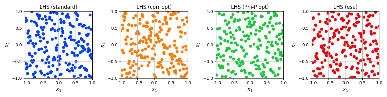
# The grid points are distributed as follows (in the normalized space):

fig, ax = plt.subplots(nrows=1, ncols=4, squeeze=True, figsize=(12.7, 3.2))

ax[0].scatter(grid_lhs_std.coords_norm[:, 0], grid_lhs_std.coords_norm[:, 1], color=sns.color_palette("bright", 5)[0])
ax[1].scatter(grid_lhs_cor.coords_norm[:, 0], grid_lhs_cor.coords_norm[:, 1], color=sns.color_palette("bright", 5)[1])
ax[2].scatter(grid_lhs_max.coords_norm[:, 0], grid_lhs_max.coords_norm[:, 1], color=sns.color_palette("bright", 5)[2])
ax[3].scatter(grid_lhs_ese.coords_norm[:, 0], grid_lhs_ese.coords_norm[:, 1], color=sns.color_palette("bright", 5)[3])

title = ['LHS (standard)', 'LHS (corr opt)', 'LHS (Phi-P opt)', 'LHS (ese)']

for i in range(len(ax)):
    ax[i].set_xlabel("$x_1$", fontsize=12)
    ax[i].set_ylabel("$x_2$", fontsize=12)
    ax[i].set_xticks(np.linspace(-1, 1, 5))
    ax[i].set_yticks(np.linspace(-1, 1, 5))
    ax[i].set_xlim([-1, 1])
    ax[i].set_ylim([-1, 1])
    ax[i].set_title(title[i])
    ax[i].grid()

plt.tight_layout()

# References
# ^^^^^^^^^
# .. [1] McKay, M. D., Beckman, R. J., & Conover, W. J. (2000). A comparison of three methods for selecting
#    values of input variables in the analysis of output from a computer code. Technometrics, 42(1), 55-61.
# .. [2] Johnson, M. E., Moore, L. M., Ylvisaker D. , Minimax and maximin distance designs,
#    Journal of Statistical Planning and Inference, 26 (1990), 131–148.
# .. [3] Morris, M. D., Mitchell, T. J. (1995). Exploratory Designs for Computer Experiments. J. Statist. Plann.
#    Inference 43, 381-402.
# .. [4] Jin, R., Chen, W., Sudjianto, A. (2005). An efficient algorithm for constructing optimal
#    design of computer experiments. Journal of statistical planning and inference, 134(1), 268-287.

# When using Windows you need to encapsulate the code in a main function and insert an
# if __name__ == '__main__': guard in the main module to avoid creating subprocesses recursively:
#
# if __name__ == '__main__':
#     main()